Introduction and setup

Overview

Teaching: 15 min
Exercises: 15 min

Questions

What will we be learning?

How will we be learning?

Objectives

Review schedule

Set expectations for engagement and behavior

Introduce ourselves

Acknowledgement of country

We wish to acknowledge the custodians of the land we reside on, for the developers of these lessons, these are the Wadjuk (Perth region) people of the Nyoongar nation. We would like to pay our respect to their Elders past, present and emerging and we acknowledge and respect their continuing culture and the contribution they make to the life of this city and this region.

Schedule

AEST	AWST	Event
09:30	07:30	Introduction and setup
10:00	08:00	Scientific Computing
11:00	09:00	break
11:30	09:30	Best Practices In Computing
12:30	10:30	break
13:30	11:30	Data Management
14:30	12:30	break
15:00	13:00	Project Management
16:00	14:00	end

Content

This workshop is designed to give you training in a broad range of skills that will be useful for your career in academia and beyond. We are not aiming to provide a deep dive into any of the material covered here, but instead will focus on making sure that everyone comes away with enough information to know what skills are useful, what questions to ask, and where to go for more information.

If you are interested in further engagement please see the links within the lessons, the bonus content lesson (not part of the HWSA workshop), chat to us in the breaks, or reach out via email or slack to get some more advice from the ADACS team.

Engagement

This workshop is developed for three main delivery methods:

Facilitated, in person, at the HWSA venue in Tasmania
Facilitated, online, in parallel with (1)
Self-paced, online, via this website.

For the HWSA school we will set up a shared google doc for people to contribute to as we go along. This means that contributions can be anonymous and asynchronous as needed. Whilst we have ADACS people here to facilitate the workshop, we encourage people to ask for help from their peers, and to offer help to those that may need it.

This workshop is all about learning by doing. We will be engaging in live coding type exercises for most of the workshop, and we will set challenges and exercises for you to complete in groups. The more you engage with your fellow learners and the more questions that you ask, the more that you will get out of this workshop.

We will be using sticky notes for in-person participants to indicate their readiness to move on: please stick them on your laptop screen to indicate if you need help or are done and ready to move ahead. For those joining online we’ll be using the cross or check icons (zoom) to indicate the same.

We will use a shared document (etherpad) to manage and record many of our interactions.

Conduct

This workshop will be an inclusive and equitable space, which respects:

the lived experience of it’s attendees,
the right for all to learn, and
the fact that learning means making mistakes.

We ask that you follow these guidelines:

Behave professionally. Harassment and sexist, racist, or exclusionary comments or jokes are not appropriate.
All communication should be appropriate for a professional audience including people of many different backgrounds.
Sexual or sexist language and imagery is not appropriate.
Be considerate and respectful to others.
Do not insult or put down other attendees.
Critique ideas rather than individuals.
Do not engage in tech-shaming.

See the ASA2022 code of conduct and the Software Carpentries code of conduct for more information.

Introduce yourselves

Introduce yourself to your peers by telling us your name, a game you enjoy playing, and a food that you would like to try but never have.

Please also introduce yourself in more detail in the shared google doc.

Key Points

This is not a lecture

The more you engage the more you will benefit

Everyone is here to learn and that means making mistakes

Scientific Computing

Overview

Teaching: 30 min
Exercises: 30 min

Questions

What is scientific computing?

How can I automate common tasks?

What is reproducible research?

Objectives

Feel good about your computing goals

Appreciate various levels of automation

Understand what reproducibility means

Scientific Computing

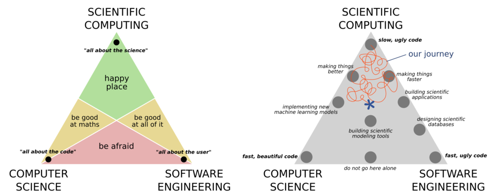
Scientific computing is best understood by its relation to, and difference from, computer science, and software engineering. Computer science places a big focus on correctness of the code and the efficiency of the algorithm. Software engineering places a big focus on the usability of the software, and how it fits within an ecosystem of other solutions. Scientific computing cares little for any of these concerns, and is primarily concerned with producing correct scientific results. There is of course a large overlap between the three ideals as shown in the ternary diagrams below.

scicomp-ternary

It is rare today that you can work on any project without having to some kind of computing. Many physics and astronomy students are not required to take any computing courses as part of their undergrad (though many do). Thankfully this is changing, however the courses are often focused on software engineering or computer science rather that scientific computing.

Your computing journey

In small groups, briefly share your computing journey, and where you feel that you currently sit in the above diagram.

As you discuss make notes in our shared document along the following topics:

When writing code or developing software, what is your primary concern?

What formal training have you had?

What are some good resources for self/peer learning?

What languages / tools do you commonly use or find particularly useful?

A key takeaway from the above is that you should not hold yourself to the standards of a computer scientist or a software engineer because you are neither of these things. Your goal is not to make software that is widely usable, highly performant, or scalable. First and foremost you are focusing on getting the science correct, and the rest is a bonus. Having said this, there is of course a large overlap between the three disciplines and some important lessons that we can take from software engineers and computer scientists that will make our science results more robust, more easy to replicate, easier to adapt and reuse, as well as allowing us to take on larger projects with more ambitious goals. This will be the focus of our first two lessons today.

Automate your way to success

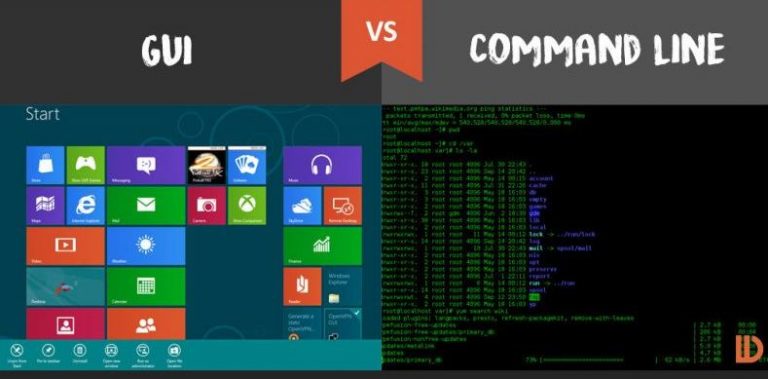
Most of the activity in which we engage on a daily basis in research is computer based. A typical researcher will use a combination of graphical and command line user interfaces (GUIs and CLIs) to interact with this software. Each have their tradeoffs and strengths, but a major difference is that it is often easy to automate programs that have a command line interface, whilst it is difficult to do the same with a graphical interface.

guivscli

Your day-to-day sciencing workflow

Think of the tasks that you do as part of your daily science-ing, and the tools that you use to make this happen. Discuss the following with your colleagues and then write in the shared document.

Match your activity to a tool that you use, or one that you want to use.

For each of the tools that you have identified note if it has a GUI or CLI (or both).

What aspects of your day-to-day do you wish you could automate?

In our shared document contribute one item from each of the above.

Simple tasks are often the most easily automated. For example, maybe you want to back up the data on your (linux) computer and you have purchased an additional hard drive for this very purpose. Due to previous bad experience with RAIDed hard drives, an aversion to over complicated software solutions, and no interest in offsite or incremental backups, you have decided that your backup and recovery will consist of copying files from one hard drive to another on a regular basis. For this task you put a reminder in your calendar every monday to execute the following code:

rsync -av --delete /data/working/${USER} /data/backup/${USER}

This will use the rsync program to copy data from the hard drive mounted at /data/working/${USER} to the one mounted at /data/backup/${USER}. Here ${USER} is the bash variable which refers to your username. The options -av will preserve the file ownership, permissions, and access date/time, and --delete will make sure that files that are in the working directory but not in the backup directory will be deleted. Essentially this will create an exact mirror of one drive onto another. The program rsync is smart enough to do this mirroring by only copying the changes from one drive to another so that you don’t have to delete and re-copy the data every week.

Challenge

What are some of the draw backs in using this method of backup?

How could you ensure that you use the same command each time you do your backup?

How could you automate this task so that you no longer have to think about it or spend time on it?

Solution notes

If you don’t have your calendar open you might forget to run the program.

You might not run the program on every Monday because you don’t work every Monday.

Keep the above text in a file called backup_instructions.txt so that you remember how to do it correctly.

Convert backup_instructions.txt into do_backup.sh, add a #! (shebang) line, and make the file executable, so you can type ./do_backup.sh

You could automate by adding the above line to your crontab so that it will always run on a Monday morning without your input

Any work that you can do from the command line can be automated in a similar way. A good approach to take when considering automating a task is:

Complete the task manually, using the command line
Copy all the commands that you used into a file so that you have an exact record
Save the file as a .sh (OSX/Linux) or .bat file (Windows)
You now have an automation script!
Next time you need to do said task, just run the script

Optional extras to make your automation even better include:

Adding some command line arguments to your script so that you can do slightly different things each time
Generalize the script so that information that may need to change between runs can be automatically generated or calculated

The Linux ecosystem is built on the idea of having a large number of tools each with a very specific purpose. Each tool should do one thing and do it well. There are many seemingly simple tools that already exist on your Linux (and OSX, or WSL) computer that you can chain together to great effect.

Favorite tools

Discuss with your group some of the command line tools that you use most often.

Let people know what tool you wish existed (because it might already!).

Share your thoughts in our shared document.

Have a look at the with list of others and see if you can propose a solution or partial solution.

Let’s explore some of these useful command line tools that you might use to provide some low-level automation to your life.

grep
wget
curl
sed
cut
wc
bc

We’ll explore these together, but if at a later point you want more help on these tools you can:

use program help via the --help flag
use manual pages like this man grep, man cut, or even man man
ask dr google

Reproducible research

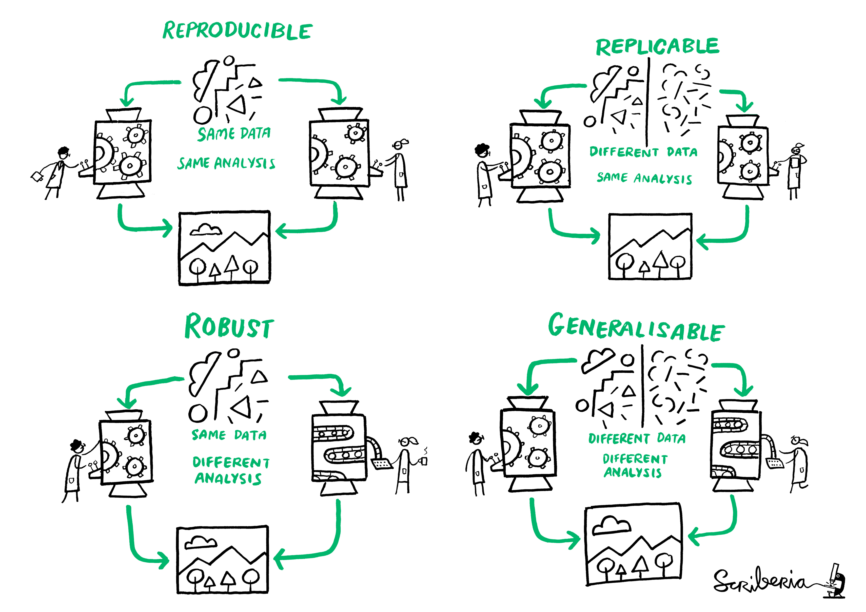
Reproducibility is the idea of being able to re-run your analysis with the same data and get the same results. Related concepts are replicability, robustness, and generalisabiltiy, as demonstrated in the following diagram.

reproduciblescience

There are many reasons why you would re-run your analysis or data processing:

As you develop your data collection, processing, and analysis techniques you will make changes to the process. Each change means re-doing all the work again.
Your work may be extended or expanded as new data become available, requiring you to apply the same processing to different data,
During the publication review process you need to make adjustments to the data selection or processing based on collaborator or referee’s comments,
Other people may want to apply your techniques to their data and compare results.

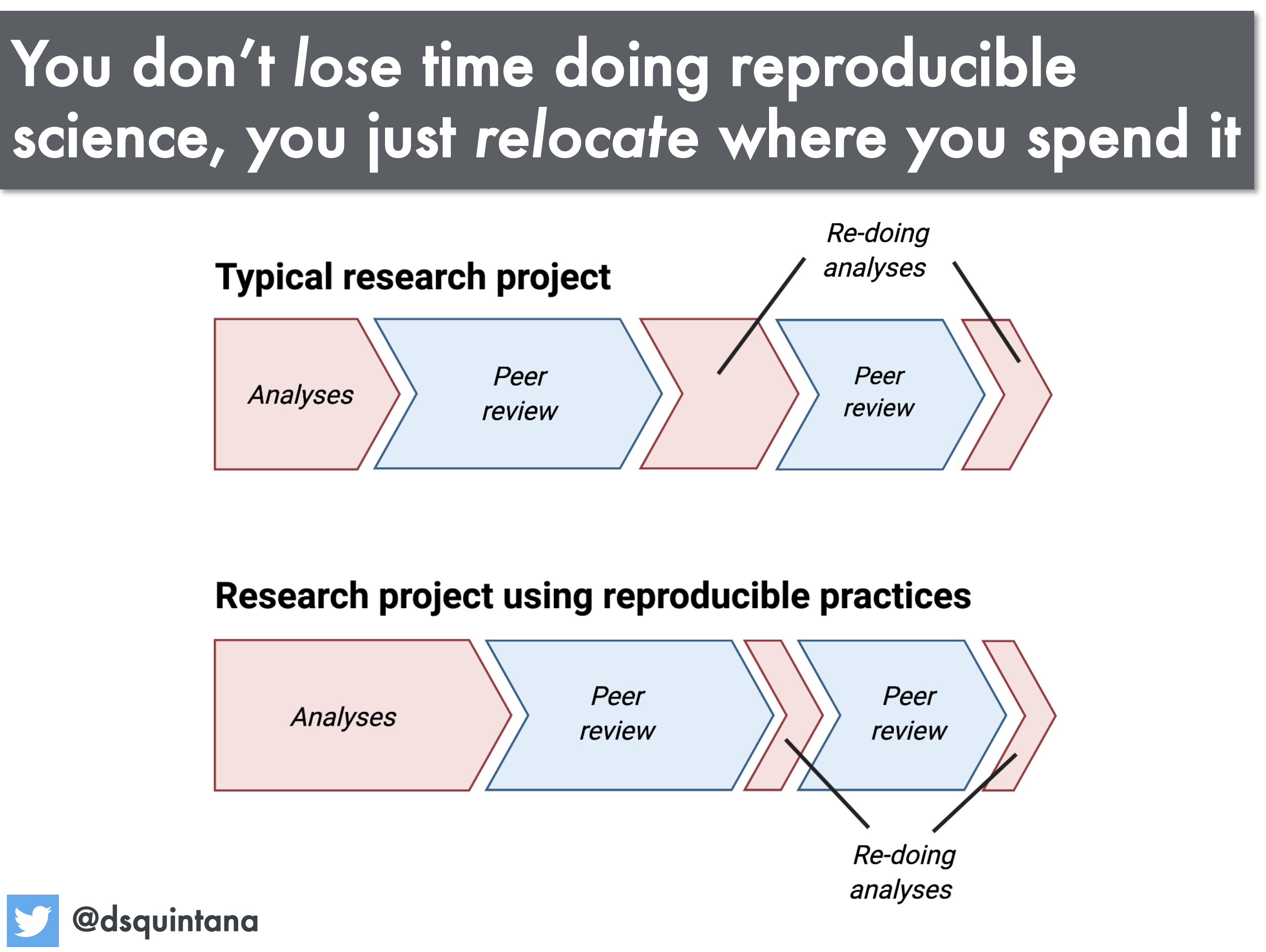
A science workflow that can be consistently re-run and easily adapted is of huge benefit to you, the researcher. Sharing your data, and your methodology (via code and documentation) with others can also benefit the community because it will allow your work to be rerun and adapted, saving others time whilst generating citations and accolades for you.

researchtime

Discussion

If you were to redo all your data processing from scratch, how confident are you that you would get the same result?

What aspects of your workflow have you automated?

What parts of your workflow cannot be automated, and what can you do about that?

Is automation essential for reproducible research?

As always, share your thoughts with your group and then put some notes into the shared document.

Key Points

Scientific computing has different goals from computer science and software engineering

You are a scientist, your focus is on the science

Automation can occur at many levels

Reproducibility is good for everyone (especially you)

Morning Tea

Overview

Teaching: min
Exercises: min

Questions

Objectives

Time for our first break.

Key Points

Best Practices In Scientific Computing

Overview

Teaching: 30 min
Exercises: 30 min

Questions

What does best practice mean?

What should I be doing?

What should I try to avoid?

Objectives

Appreciate guidelines for best practice

Work through an exercise demonstrating some of these practices

Be less scared about testing and documentation

Best Practices In Scientific Computing

While computer science and software engineering have different goals than scientific computing, many of the best practices in these disciplines are still applicable to scientific computing.

Since the top priority of scientific computing is to have software that produces correct results, we can make our lives easier by adopting practices that make our code or scripts easier to understand (by humans) so that errors can be found and fixed easily. Additionally, since our research work is continuously changing it is very likely that we will revisit our scripts to re-use them (in part or in whole) or expand their use. Here again readability and clarity will be of benefit, but so will version control, and modularization.

Here are some guiding principles that should be followed when planning or writing scripts, regardless of language:

Guideline	Description
Clarity over efficiency	Prioritize writing clear code over efficient code. Make use of programming idioms¹. Do standard things in standard ways. Write code for humans to understand in the first instance, and only secondarily for computers.
Naming is important	Choose meaningful and useful names for variables/functions/classes/scripts. Typically: objects are nouns, functions are verbs, pluralize variables that represent lists or collections. Unhelpful names can be annoying to work with, whilst confusing names can be downright destructive.
Don’t repeat yourself	When something works reuse it. Bundle repeated code into functions and call those functions. Bundle functions into modules that can be imported. Write simple (single intent) tools that can be easily incorporated into larger workflows.
Don’t repeat others	If something seems routine then there is almost always an existing solution that you can rely on. Look for existing libraries/modules or programs that you can make use of. Don’t reinvent the wheel²
Document	You will forget what you did and why you did it. Write yourself a document that describes the problem you were trying to solve, the approach that you took, and how you solved it. If the solution is a script, then describe how to use the script including the inputs, what options are available, and what the output is. This can be a `README.md` file, docstrings (in python) or a pdf. The format is less important than the fact that the documentation exists.
Test	Only the very lucky get things right the first time. Don’t rely on luck. When you write a script, do something to convince yourself that it works. Manually inspecting results for a known example is form of testing. This of testing as validation.
Version control	When moving towards a solution we often make a wrong turn. Use a version control system to create a ‘checkpoint’ or ‘save point’ that you can easily come back to if things go bad. You don’t need to do pull requests, branching, merging, or upload your files to GitHub for version control to be useful.
Avoid premature optimization	Optimization can save time in the term run but always costs time in the short term. Optimize your time by firstly solving the problem, and only engage in optimization after you find out that your code is taking too long or using too many resources³.

In this lesson we will focus on repetition, version control, testing, documentation, and repetition. To demonstrate the utility of these topics we’ll be working on a common task - analyzing meteorite falls around the world.

Use case - visualizing a data set

Let’s go through the process of visualizing some data and see if we can incorporate the above best practices as we go. We will be working with a data file that contains information about meteorites that have fallen in Australia, and our aim is to plot the location of the meteorites, and give an indication of their masses.

To begin with we need to obtain the data. We have a nice data set prepared for you which you can download the data with the command⁴:

wget https://raw.githubusercontent.com/ADACS-Australia/HWSA-2022/gh-pages/data/Australian_Meteorite_Landings.csv
# or if the above didn't work, then try
curl -O https://raw.githubusercontent.com/ADACS-Australia/HWSA-2022/gh-pages/data/Australian_Meteorite_Landings.csv

We will start with a peak inside this file with the head command:

head Australian_Meteorite_Landings.csv

output

id,mass (g),reclat,reclong
5051,488.1,-33.15639,115.67639
48653,324.0,-31.35,129.19
7743,30.0,-31.66667,152.83333
10033,127.0,-29.46667,151.61667
10120,26000.0,-33.35,146.85833
12264,41730.0,-35.08333,139.91667
16643,330000.0,-26.45,120.36667
16738,8887.5,-40.975,145.6
16766,11300.0,-29.8,141.7

From this you can see that we have given you a .csv file recording meteorites that have landed in Australia. The four columns represent an ID, a mass, and a recorded position in latitude and longitude.

We’ll use python for our visualization, so we begin by reading the file with python. Reproducing the above quick summary in python we would write a script like the following:

# the csv library has a lot of read/write functions for csv files
import csv

csv_list = []

# opening the CSV file
with open('Australian_Meteorite_Landings.csv', mode ='r') as file:
  # read the CSV file
  csv_reader = csv.reader(file)

  # loop over the lines in the file and add each to our list
  for line in csv_reader:
        csv_list.append(line)

# print the first 10 lines to ensure that we are on the right track.
print(csv_list[:10])

output

[['id', 'mass (g)', 'reclat', 'reclong'], ['5051', '488.1', '-33.15639', '115.67639'], ['48653', > '324.0', '-31.35', '129.19'], ['7743', '30.0', '-31.66667', '152.83333'], ['10033', '127.0', '-29.> 46667', '151.61667'], ['10120', '26000.0', '-33.35', '146.85833'], ['12264', '41730.0', '-35.08333', > '139.91667'], ['16643', '330000.0', '-26.45', '120.36667'], ['16738', '8887.5', '-40.975', '145.6'], > ['16766', '11300.0', '-29.8', '141.7']]

At this point we should save our work in a file and make sure that we are on the right track by running the script and inspecting the output. Since we have just started our new project and have some initial progress, this is a great time to set up our version control.

Start a new project

Create a new directory for your project with a name that makes sense to you

Save your initial python script as plot_meteorites.py (what we’ll eventually be doing)

Run your script and ensure that it’s not broken

Initialize a git repository in this directory by typing git init

Tell git that you want this new file to be tracked by using git add <filename>

Also commit your data file using the same technique

Save your initial progress by creating a new commit to your repository via git commit -m > <message>

The first commit message can be something simple like “initial version”

Check that you have committed your progress by running git log

If at any point we are editing our work and we break something, or change our mind about what we are doing, so long as we have the files under version control we can go back to our previous save point using:

git checkout -- <filename>

If we want to reach way back in time we can do

git checkout <hash> <filename>

Where the <hash> is one of the long alphanumeric strings that are shown when we run git log. Having good commit messages will make it easier to tell which commit we should be going back to.

Now we have some first step that we can come back to later if we mess things up. Let’s try and do something with this data - computing the mean mass of the meteorites. We can do this by adding the following to our script and re-running:

import numpy as np

all_mass = []

# csv_list[1:] will skip the first line which is our header (not data)
for id, mass, lat, long in csv_list[1:]:
    # skip missing data
    if mass != "":
        # Convert string -> float and append to our list
        all_mass.append(float(mass))

# Output mean of the masses
print("The mean mass is:", np.mean(all_mass), "g")

...
The mean mass is: 80919.38811616955 g

Save your progress

Once our script is in a working state, save it, add it to git, and then commit it

Use a commit message that describes what we did in less than 50 chars

Double check your git log to see that the changes have been applied

The above is fine but that was a bit of work for what feels like a very standard task. Let’s be guided by the “don’t repeat others” mentality, and see if we can find an existing solution that will do this work for us. The python data analysis library pandas has a lot of great functionality built around data structures called data frames which are a fancy kind of table. So if we let pandas do all the hard work for us then we can extend our above code with the following:

# Use the pandas library
import pandas as pd

# read a csv file into a data frame
df = pd.read_csv('Australian_Meteorite_Landings.csv')

# Have a look at the data
print("csv data\n--------------------------")
print(df)

# Use pandas to do some quick analysis
print("\npanda describe\n--------------------------")
print(df.describe())

output

...
csv data
--------------------------
        id   mass (g)    reclat    reclong
0     5051      488.1 -33.15639  115.67639
1    48653      324.0 -31.35000  129.19000
2     7743       30.0 -31.66667  152.83333
3    10033      127.0 -29.46667  151.61667
4    10120    26000.0 -33.35000  146.85833
..     ...        ...       ...        ...
638  30359      262.5 -32.03333  126.17500
639  30361   132000.0 -14.25000  132.01667
640  30362    40000.0 -31.19167  121.53333
641  30373   118400.0 -29.50000  118.75000
642  30374  3800000.0 -32.10000  117.71667

[643 rows x 4 columns]

panda describe
--------------------------
                 id      mass (g)      reclat     reclong
count    643.000000  6.370000e+02  643.000000  643.000000
mean   19219.513219  8.091939e+04  -30.275400  130.594478
std    14869.941958  1.029442e+06    2.940091    7.655877
min      471.000000  0.000000e+00  -41.500000  114.216670
25%    10136.500000  3.280000e+01  -30.841665  126.587915
50%    15481.000000  1.291000e+02  -30.383330  128.916670
75%    23537.500000  2.426000e+03  -30.086415  132.008335
max    56644.000000  2.400000e+07  -12.263330  152.833330

With only a few lines we can load the data and have a quick look. You can see that the count of mass is only 637 out of 643 so pandas has recognized that there is missing mass data and has even calculated a mean mass for us.

Save your progress

Once our script is in a working state, save it, add it to git, and then commit it

Use a commit message that describes what we did in less than 50 chars

Double check your git log to see that the changes have been applied

Now that pandas is doing all the file reading and format handling for us we can do away with our previous attempt at reading a csv file.

Delete some code and check it in

Delete all the code before the “import pandas as pd” command

Run git status to see which files have changed

Run git diff plot_meteorites.py to see what changes have been made to the file

Run the script and confirm that it still works

Add and commit our work to our git repository

Pre-existing solutions

See if you can identify a python package (module) that will help you with each of the following tasks:

Read .fits format images

Create a ‘corner plot’ from multi-dimensional data

Plot images using sky coordinates using the correct projection

Read and write .hdf5 format data files

Solve equations analytically/exactly

Train and evaluate machine learning models

Head over to the python package index at pypi.org, and search for the packages you found.

In our shared document make a note of a package that you wish existed, and then look at the wish list of others and see if you can suggest a (partial) solution.

In the above challenge you may have seen a few modules that occur frequently, either because they are large and multi-purpse modules, or because they are fundamental and used as a building block for many others. For example, scipy and numpy are fundamental to most of the scientific computing libraries that are built, and packages like astropy are becoming very widely use in astronomy.

If you have noticed a bias towards python in our teaching examples, it is because of this rich ecosystem of freely available and easy to use modules. The large adoption within the astronomy community, also means that it is easy to get relevant and specific help from your peers. As you work in other fields you’ll notice that different software packages are standard and usually for the same reason - easy of access, and access to support. At the end of the day the right tool is the one that gets the job done, and you should not be afraid of exploring beyond python to get your work done.

Visualizing data

Back to our main task of making a nice plot of our data. Let’s make a scatter graph of the locations of the meteorites using the matplotlib module.

Since this should be a simple task, we shouldn’t be supprized to find that we can complete it in a few lines of code. Add the following to our script and run it:

# import the plotting library with a short name
import matplotlib.pyplot as plt

# make a scatter plot
plt.scatter(df['reclong'], df['reclat'], edgecolors='0')

# label our plot!
plt.xlabel("Longitude (deg)")
plt.ylabel("Latitude (deg)")
plt.title("Meteorite landing locations")

# pop up a window with our plot
plt.show()

Our first plot

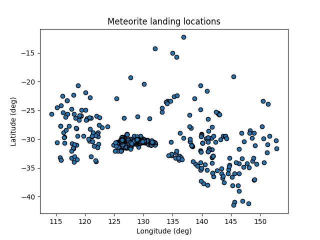
Save your progress

Commit your changes to the plotting script.

Our plot looks vaguely Australia shaped but to be sure lets plot this against a map of Australia to make sure we believe the locations. Doing this manually would be difficult so, after some Googling, we have found a python module that can do it for you called Basemap

Replace the previous plotting section of your script with the following:

from mpl_toolkits.basemap import Basemap
import numpy as np
import matplotlib.pyplot as plt

fig=plt.figure()

# setup map projection
bm = Basemap(
    llcrnrlon=df['reclong'].min()-5,  # Lower left corner longitude
    urcrnrlon=df['reclong'].max()+5,  # Upper right corner longitude                   
    llcrnrlat=df['reclat'].min()-5,   # Lower left corner latitude
    urcrnrlat=df['reclat'].max()+5,   # Upper right corner latitude
)

# Draw in coasline and map lines
bm.drawcoastlines()
bm.fillcontinents()
bm.drawparallels(np.arange(-90,90,10),  # The location of the parallels
                 labels=[1,1,0,1])      # Which axes to show labels on
bm.drawmeridians(np.arange(-180,180,10),labels=[1,1,0,1])

# Convert your data to the Basemap coordinates and add it to the plot
x, y = bm(df['reclong'], df['reclat'])
plt.scatter(x, y, 
            edgecolors='0',
            zorder=2) # make the points be in front of the basemap
plt.show()

Our second plot

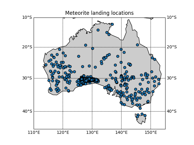
Save your progress

Commit your changes to the plotting script.

Creating a reusable script

This is looking great but before we go any further we should make the plotting component into a function as part of a script so it’s easier to rerun for different locations on the Earth. Moving commonly used code into a function, rather than just copy/pasting it, is ane example of don’t repeat yourself.

Let’s take all of the plotting part of our script and put it into a function called plot_meteor_locations, and allow the user to supply a data frame with the data, and a bounding box of lat/long for the plotting area.

Since this function is something that we’ll be using often, it’s a good idea to write some documentation for the function. In python we can use a docstring to show what the function is supposed to do and what the expected inputs ared. Alternatively we could write a short noted in a REDEME.md file that describes how to use the program.

import matplotlib.pyplot as plt
from mpl_toolkits.basemap import Basemap
import pandas as pd
import numpy as np


def plot_meteor_locations(df):
    fig=plt.figure()

    # setup map projection
    bm = Basemap(
        llcrnrlon=df['reclong'].min()-5,  # Lower left corner longitude
        urcrnrlon=df['reclong'].max()+5,  # Upper right corner longitude                   
        llcrnrlat=df['reclat'].min()-5,   # Lower left corner latitude
        urcrnrlat=df['reclat'].max()+5,   # Upper right corner latitude
    )
    
    # Draw in coasline and map lines
    bm.drawcoastlines()
    bm.fillcontinents()
    bm.drawparallels(np.arange(-90,90,10),  # The location of the parallels
                     labels=[1,1,0,1])      # Which axes to show labels on
    bm.drawmeridians(np.arange(-180,180,10),labels=[1,1,0,1])
    
    # Convert your data to the Basemap coordinates and add it to the plot
    x, y = bm(df['reclong'], df['reclat'])
    plt.scatter(x, y, 
                edgecolors='0',
                zorder=2) # make the points be in front of the basemap
    plt.show()
    return

if __name__ == '__main__':
    # read a csv file into a data frame
    df = pd.read_csv('Australian_Meteorite_Landings.csv')
    plot_meteor_locations(df)

Now you have a script that is easy to rerun if you want to recreate the plot and if anyone asks you how you generated the results you can show them your script so you can go through the steps one by one to confirm their validity.

Let’s focus on New Zealand

Verify that your code works and then commit the changes to your repo

Download the New Zealand data file

Edit your script to use the new data file, save, and rerun

Making your script re-usable

Right now if someone wants to use your script they would have to import that function into their own script like this:

from plot_meteorites import plot_meteor_locations
# ... load a data frame called df
plot_meteor_locations(df)

However, it is often nice to have a basic command line interface. In python any arguments that we pass to the program are stored in a list, and we can access this list from the sys module via sys.argv. If we want to read the name of the data file from the command line we can modify our if __main__ clause like this:

import sys

# ... the rest of our code

if __name__ == '__main__':
    # get the filename from the command line as the last argument
    csv_file = sys.argv[-1]
    # read a csv file into a data frame                     
    df = pd.read_csv(csv_file)
    plot_meteor_locations(df)

Here the sys.argv[-1] refers to the last argument that was given. It will always be interpreted as a string, and in this case we’ll use it as a filename.

add a command line interface

modify your code so that it reads the name of the data file from the command line

test your code by running it on both the Australia and New Zealand data

commit your changes to your repository (including the new data file)

Testing

Testing is something that many people think is too much work to bother with. However, we are always testing our code even if we don’t think of it that way. Any time you run your code and compare the behavior/output with expectations is a test. Testing is not hard, and we already do it so let’s just embrace that.

In the previous challenge we ran our code on two different data sets, and then inspected the output to confirm that the code was working as intended. To do that we ran the following bash commands:

python3 plot_meteorites.py New_Zealand_Meteorite_Landings.csv
python3 plot_meteorites.py Australian_Meteorite_Landings.csv

If we were to make some changes to our code, it is a good idea to re-run these tests to make sure that we haven’t broken any of the existing functionality. If we are adding some new functionality, or fixing some bug, then it would be good to have a new test to run to verify that the new parts of the code are working as intended. To remind ourselves of how we do the testing lets make a file to record the process. In fact, we can just make a file called test.txt which includes the above two lines of code and maybe a short description of what is expected. When we want to run the test we just open the file and follow the instructions, copy/paste the lines of code as required.

If we think back to our lesson on scientific computing and automation we can take this a step further. We could write test.sh with the same lines of code as test.txt (and convert the instructions into comments), and then use source test.sh to have all the code execute automatically.

As your testing becomes more involved you’ll eventually want to look into some more automated ways of not just running the tests, but ensuring that the tests all pass. For this you’ll have to come up with some quantitative measures of what pass/fail look like, and then write a bit of code that will check against these conditions. If/when you get to this point you should start thinking about using a testing framework such as pytest to help with the automation and organization of the tests. (You still have to write them yourself though!)

Create test file

Create either test.txt or test.sh using the example above

Do/run the test

Commit the test file to your git repo

Documentation

Documenting your code is important as it makes it clear how you code generates your results and shows others (and yourself) how to use your code. There are several levels of documentation and what level is appropriate depends on the purpose, complexity and who will use your code.

Documentation levels include:

Code comments
README.md
--help or docstrings (Python)
readthedocs.io which can host your documentation and using sphinx you can automate it’s generation
A user guide (pdf or markdown) to explain how to use the code with explanations and common examples

Considering your audience is a good indicator of what documentation level you should aim for

You in 6 months time (level 1-3)
Other developers of the code (level 1-4)
Other users (level 4-5)

Markdown (.md) is a common syntax to generate documentation, for example a README.md will automatically be rendered on GitHub.

Lets create a README.md for your code.

# Meteorite Analysis Software
This git repository contains python scripts to analyze meteorite data for my research, which is bound to win me the noble prize.

## Installation
This software isn't installable (yet), but it's always good to describe how to install your software. Some common ways to install python scripts include

`python setup install`

or

`pip install .`

## Data
It is always best to note where your data came from and describe how to use it.

### Australian_Meteorite_Landings.csv
Data downloaded from https://raw.githubusercontent.com/ADACS-Australia/HWSA-2022/gh-pages/data/Australian_Meteorite_Landings.csv.
A truncated version of the data from https://data.nasa.gov/Space-Science/Meteorite-Landings/ak9y-cwf9.

id: NASA meteorite

mass (g): Mass of the meteorite in grams

reclat: Recorded latitude in degrees

reclong: Recorded longitude in degrees

## Running Software
Create analysis plots using:

`python plot_meteorites.py`

You can use VSCode extensions to view the rendered version or push it to GitHub to view it on the webpage. This will remind you how to use your code and where you got your data.

Create a README file for your repo

Create a README.md file in your repo

Add your name, an description of the intent of the repo, and what the various files do

Commit this file to your git repo

See programming idioms ↩
Re-inventing the wheel can be a great learning experience, however when you are focusing on getting work done, it’s most often not a good use of your time. ↩
Consider this handy chart from xkcd ↩
wget isn’t available via gitbash, but curl is so windows users may have to use curl ↩

Key Points

Validation is testing

Documentation benefits everyone (especially you)

Version control will save you time and effort

Lunch

Overview

Teaching: min
Exercises: min

Questions

Objectives

Time for Lunch.

Key Points

Managing Data

Overview

Teaching: 30 min
Exercises: 30 min

Questions

Why do I need to manage data?

How do I manage different types of data?

How do I store and access structured data?

How do I store and access unstructured data?

Objectives

Distinguish between different types of data

Understand how to work with structured and unstructured data

Be comfortable with SQL select and filter queries

Understand what meta-data is

Managing Data

All of our research is fundamentally reliant on data so it’s important to understand the different types of data, how to store them, and how to work with them. In this lesson we’ll learn all the above!

Types of data

Fundamentally computers store data as 0s and 1s, representing floats, integers, boolean, or character data types. However this is not what we are going to talk about here. Here we are more concerned with a higher level of abstraction, which includes the following data types:

raw data
- as it comes directly from a sensor or data source
- contains signal + noise
- format and quality is highly dependent on the data source
clean data
- has bad/invalid records removed or flagged
- has been converted to a format which is usable by your analysis or processing tools
transformed data
- useful features have been identified
- low level aggregation has been applied
- instrument/sensor/model dependent effects have been removed
reduced data
- has been modeled
- has been processed into a different form such as images or a time series
published data
- the highest level of abstraction/aggregation of your data
- often represented as tables or figures

The following describes a generic data processing workflow DataProcessing

Discussion

In your groups have a look at the different types of data and stages of the data processing workflow. Think about:

Where do you get your data from?

Are there more than one source of data?

How do you keep track of which data is in which stage of processing?

When you publish your work, which data products do you want to keep and which can be deleted?

Record some notes in the shared document.

We can classify data by the processing stage as was done above, but also in an orthogonal dimension of how the data is organized. The two most general considerations here are either structured or unstructured data.

StructredUnstructredData

The way that we can store and access data depends on how it’s structured.

Structured data

One of the easiest ways to store structured data are in one or more tables. The tables themselves can be stored as .csv, .fits, or .vot tables which can be read by many astronomy software tools such as topcat. Google sheets, Microsoft Excel, or LibreOffice Calc can also be beneficial for storing structured data, particularly because they allow you to do some data exploration, cleaning, filtering, and analysis within the file itself.

When your data volumes become large, or you find yourself needing to have multiple related tables, then you probably want to start exploring databases as a storage option. See the Bonus Content

Unstructured data

Unstructured data cannot be aggregated or combined into a single data format due to their lack of common structure. In such cases it is often best to make use of a regular directory/file structure to store the individual files in a way that can be navigated easily. A well planned directory/file structure it is very useful to store meta-data about each of the files that you are storing. For example you could have:

A README.md file in the root directory that describes the directory/file structure
A metadata.csv file that maps the location of a file to some high level information such as the file format, the date the file was collected, the processing stage of the data, or the version of the file.

Exercise

Download example data example.zip

Unzip the file and have a look at the content

See if you can infer the purpose of each file

Make a plan for how you would store and manage this data

Note in the shared document what you have decided for at least one of the files

Data cleaning

In the previous lesson we worked with a file Australian_Meteorite_Landings.csv. For your benefit this had already been cleaned to remove invalid entries, attributes that we didn’t need, and entries that were not relevant.

Let’s now start with the original data set and go through the cleaning process.

wget -O Meteorite_Landings.csv https://data.nasa.gov/api/views/gh4g-9sfh/rows.csv?accessType=DOWNLOAD
# or
curl -o Meteorite_Landings.csv -O https://data.nasa.gov/api/views/gh4g-9sfh/rows.csv?accessType=DOWNLOAD

Now we’ll explore the data set using pandas.

View the raw data

Using your viewer of choice, have a look at the csv file that we just downloaded. Think about and discuss:

Are there any missing data?

What can be done about the missing data?

Are there any columns that are not useful?

Note in our shared document which tool you used to inspect the data, and one that you would take to clean this data.

Solution with pandas

import pandas as pd
df = pd.read_csv('Meteorite_Landings.csv')
print("Quick look of data")
print(df)
print("Summary of data")
print(df.describe())

Quick look of data
             name     id nametype              recclass  mass (g)   fall    year    > reclat    reclong             GeoLocation
0          Aachen      1    Valid                    L5      21.0   Fell  1880.0  50.> 77500    6.08333       (50.775, 6.08333)
1          Aarhus      2    Valid                    H6     720.0   Fell  1951.0  56.> 18333   10.23333    (56.18333, 10.23333)
2            Abee      6    Valid                   EH4  107000.0   Fell  1952.0  54.> 21667 -113.00000      (54.21667, -113.0)
3        Acapulco     10    Valid           Acapulcoite    1914.0   Fell  1976.0  16.> 88333  -99.90000       (16.88333, -99.9)
4         Achiras    370    Valid                    L6     780.0   Fell  1902.0 -33.> 16667  -64.95000     (-33.16667, -64.95)
...           ...    ...      ...                   ...       ...    ...     ...       ..> .        ...                     ...
45711  Zillah 002  31356    Valid               Eucrite     172.0  Found  1990.0  29.> 03700   17.01850       (29.037, 17.0185)
45712      Zinder  30409    Valid  Pallasite, ungrouped      46.0  Found  1999.0  13.> 78333    8.96667     (13.78333, 8.96667)
45713        Zlin  30410    Valid                    H4       3.3  Found  1939.0  49.> 25000   17.66667       (49.25, 17.66667)
45714   Zubkovsky  31357    Valid                    L6    2167.0  Found  2003.0  49.> 78917   41.50460     (49.78917, 41.5046)
45715  Zulu Queen  30414    Valid                  L3.7     200.0  Found  1976.0  33.> 98333 -115.68333  (33.98333, -115.68333)

[45716 rows x 10 columns]
Summary of data
                 id      mass (g)          year        reclat       reclong
count  45716.000000  4.558500e+04  45425.000000  38401.000000  38401.000000
mean   26889.735104  1.327808e+04   1991.828817    -39.122580     61.074319
std    16860.683030  5.749889e+05     25.052766     46.378511     80.647298
min        1.000000  0.000000e+00    860.000000    -87.366670   -165.433330
25%    12688.750000  7.200000e+00   1987.000000    -76.714240      0.000000
50%    24261.500000  3.260000e+01   1998.000000    -71.500000     35.666670
75%    40656.750000  2.026000e+02   2003.000000      0.000000    157.166670
max    57458.000000  6.000000e+07   2101.000000     81.166670    354.473330

solution with bash

head Meteorite_Landings.csv

name,id,nametype,recclass,mass (g),fall,year,reclat,reclong,GeoLocation
Aachen,1,Valid,L5,21,Fell,1880,50.775000,6.083330,"(50.775, 6.08333)"
Aarhus,2,Valid,H6,720,Fell,1951,56.183330,10.233330,"(56.18333, 10.23333)"
Abee,6,Valid,EH4,107000,Fell,1952,54.216670,-113.000000,"(54.21667, -113.0)"
Acapulco,10,Valid,Acapulcoite,1914,Fell,1976,16.883330,-99.900000,"(16.88333, -99.9)"
Achiras,370,Valid,L6,780,Fell,1902,-33.166670,-64.950000,"(-33.16667, -64.95)"
Adhi Kot,379,Valid,EH4,4239,Fell,1919,32.100000,71.800000,"(32.1, 71.8)"
Adzhi-Bogdo (stone),390,Valid,LL3-6,910,Fell,1949,44.833330,95.166670,"(44.83333, 95.> 16667)"
Agen,392,Valid,H5,30000,Fell,1814,44.216670,0.616670,"(44.21667, 0.61667)"
Aguada,398,Valid,L6,1620,Fell,1930,-31.600000,-65.233330,"(-31.6, -65.23333)"

wc Meteorite_Landings.csv

  45717  166894 3952161 Meteorite_Landings.csv

You may have noticed when inspecting the file above, that the header names are occasionally useful, but don’t do a good job of explaining what the data represent. For example:

what does the “rec” in reclat/reclong represent?
Why do some meteors have blank reclat/reclon, while others have (0,0)?
- Did someone found a meteorite at the Greenwich observatory?
There are many meteorites with the same reclat/reclong, why is this?
What does recclass represent?

Here is where we need to think about the meta-data attached to this table. We need context (how/why the table was created), and also a description of what the data represent. If we go to the NASA website which provides this data, they have a description of the column data. However, it’s not so helpful:

MeteoriteColumnDescriptions

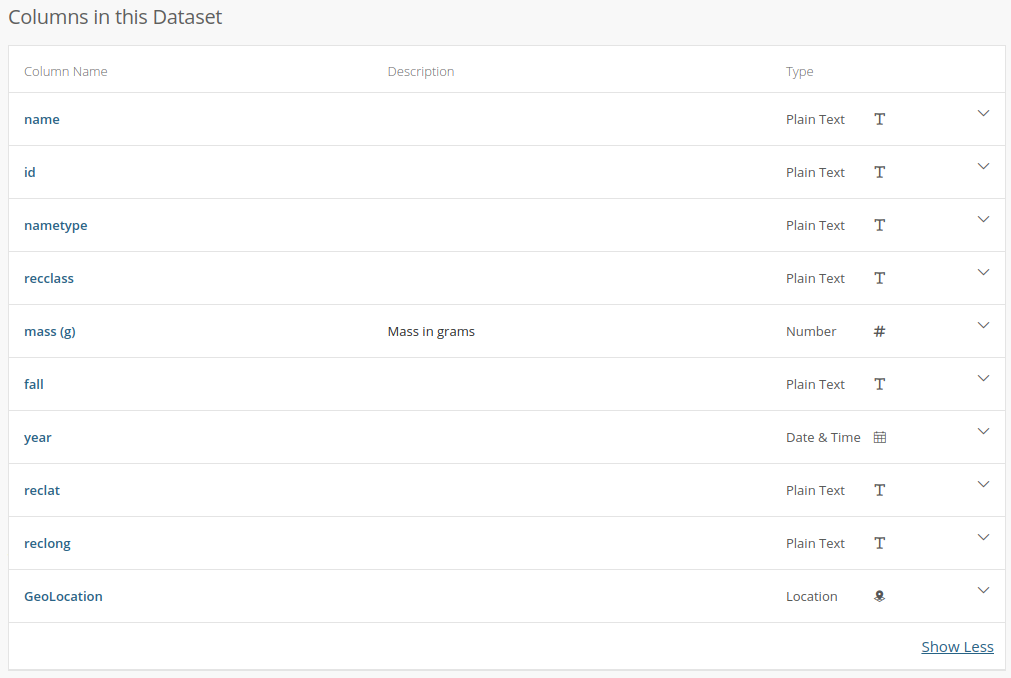
Wuh-wah! The only column with a description is the one that was most obvious. Not only that, but the data type listed for the columns is incorrect in many cases. For example, id, reclat, and reclat are listed as being “plain text” but they are clearly numeric (int, and floats), while “year” is listed as being “date and time”.

Enough complaining, lets start fixing.

Challenge

We want to plot all the Australian meteorites, with a measured mass value, and a nametype of “Valid”

Using pandas, load the meteorite dataset

Delete the geolocation column as it’s a duplicate of the reclat/reclong columns

Select all rows with a non-zero and non-null mass value

Count the rows and record this number

Delete these rows

Repeat the above for:

rows with a reclat/reclong that are identically 0,0

rows with a blank reclat/reclong

rows with nametype that is not “Valid”

Delete the nametype column as it’s now just has a single value for all rows

Choose a bounding box in lat/long for Australia (don’t forget Tassie!)

Select, count, and delete all rows that are outside of this bounding box

Save our new dataframe as a .csv file

Run our previously created script on this file and view the results

Data storage and access

The way that you store and access data depends on many things including the type of data, the structure of the data, and the ways that you will access and use the data.

We’ll focus here on the two data types introduced at the start of this lesson: structured and unstructured data.

Structured data

These are the kinds of data that we can store as rows in a .csv file or Excel spreadsheet. The two options for storing these data would be flat files or a database. A flat-file is, as the name suggests, a single file which contains all the information that you are storing. You need an independent program to load/sort/update the data that is stored in a flat-file. As the data volume becomes large, or the relation between data in different flat-files becomes more intertwined the creation, retrieval and management of these files can become time consuming and unreliable.

A database is a solution that combines the data storage, retrieval, and management in one program. A database can allow you to separate the way that the data are stored logically (tables and relations) and physically (on disks, over a network).

We’ll explore some basics of data bases using sqlite3. This program supports the core functionality of a relational database without features such as authentication, concurrent access, or scalability. For more advanced features you can use more full featured solutions such as PostgreSQL or MySQL. One of the nice things about sqlite3 is that it stores all the data in a single file, which can be easily shared or backed up. For this lesson we’ll be working with a ready made database Meteorite_Landings.db.

Using SQL to select data

There are two choices of how you can use sqlite3 for this lesson:

run sqlite3 Meteorite_Landings.db from your terminal
Go to sqliteonline.com and upload the file

The data in a database is stored in one or more tables, each with rows and columns. To view the structure of a table we can use:

.schema

CREATE TABLE IF NOT EXISTS "landings" (
"index" INTEGER,
  "name" TEXT,
  "id" INTEGER,
  "nametype" TEXT,
  "recclass" TEXT,
  "fall" TEXT,
  "year" REAL,
  "reclat" REAL,
  "reclong" REAL,
  "GeoLocation" TEXT,
  "States" REAL,
  "Counties" REAL,
  "mass" REAL
);

What we see in the output here are the instructions on how the table was created. The name of the table is landings, and there are a bunch of column names which we recognize from previous work. We can see that each column has a particular data type (TEXT, INTEGER, REAL). In a database the types of data that can be stored in a given column are fixed and strictly enforced. If you tried to add “one” to a column with type REAL, then the database software would reject your command and not change the table.

If we want to see the content of the table, we need to SELECT some data. In SQL we can do this using the SELECT command as follows:

SELECT <columns> FROM <table>;
SELECT name, mass, year FROM landings;
SELECT * FROM landings;

The last command is the most common command for just looking at the table content as it will show all the columns without you having to list them all. If we want to show only the first 10 lines (like head) then we can choose a LIMIT of lines using:

SELECT * FROM landings LIMIT 10;

Note that if you are using the command line version of sqlite3 the default output can be a little hard to read. Firstly, you’ll get all the data speeding by. Secondly, the data are not well formatted for humans to read. We can fix this with a few commands:

.mode column
.headings on

Combining all this together we have the following:

sqlite> SELECT * FROM landings LIMIT 10;

index       name        id          nametype    recclass    fall        year        reclat      reclong     GeoLocation        States      Counties    mass      
----------  ----------  ----------  ----------  ----------  ----------  ----------  ----------  ----------  -----------------  ----------  ----------  ----------
         Aachen      1           Valid       L5          Fell        1880.0      50.775      6.08333     (50.775, 6.08333)                          21.0      
         Aarhus      2           Valid       H6          Fell        1951.0      56.18333    10.23333    (56.18333, 10.233                          720.0     
         Abee        6           Valid       EH4         Fell        1952.0      54.21667    -113.0      (54.21667, -113.0                          107000.0  
         Acapulco    10          Valid       Acapulcoit  Fell        1976.0      16.88333    -99.9       (16.88333, -99.9)                          1914.0    
         Achiras     370         Valid       L6          Fell        1902.0      -33.16667   -64.95      (-33.16667, -64.9                          780.0     
         Adhi Kot    379         Valid       EH4         Fell        1919.0      32.1        71.8        (32.1, 71.8)                               4239.0    
         Adzhi-Bogd  390         Valid       LL3-6       Fell        1949.0      44.83333    95.16667    (44.83333, 95.166                          910.0     
         Agen        392         Valid       H5          Fell        1814.0      44.21667    0.61667     (44.21667, 0.6166                          30000.0   
         Aguada      398         Valid       L6          Fell        1930.0      -31.6       -65.23333   (-31.6, -65.23333                          1620.0    
         Aguila Bla  417         Valid       L           Fell        1920.0      -30.86667   -64.55      (-30.86667, -64.5                          1440.0    

By convention we use all caps for the keywords, and lowercase for table/column names. This is by convention only, and sqlite3 is not case-sensitive.

We can filter the data that we retrieve by using the WHERE clause.

SELECT <columns> FROM <table> WHERE <condition> LIMIT 10;

Challenge

Find all the meteorites that fell between 1980 and 1990, and have a mass between 100-1,000g.

List the name and reclat/reclong for 15 of these meteorites

Solution

sqlite> SELECT name, reclat, reclong FROM landings WHERE year >= 1980 AND year <=1990 LIMIT 15;

name        reclat      reclong   
----------  ----------  ----------
Akyumak     39.91667    42.81667  
Aomori      40.81056    140.78556 
Bawku       11.08333    -0.18333  
Binningup   -33.15639   115.67639 
Burnwell    37.62194    -82.23722 
Ceniceros   26.46667    -105.23333
Chela       -3.66667    32.5      
Chiang Kha  17.9        101.63333 
Chisenga    -10.05944   33.395    
Claxton     32.1025     -81.87278 
Dahmani     35.61667    8.83333   
El Idrissi  34.41667    3.25      
Gashua      12.85       11.03333  
Glanerbrug  52.2        6.86667   
Guangnan    24.1        105.0     

You can interact with a database programmatically using the python module sqlite3. With the combination of sqlite3 and pandas modules, you can save a pandas data frame directly to a database file. This is one of the easiest ways to create a simple database file.

import sqlite3 as sql
import pandas as pd

# read the .csv file
df = pd.read_csv("Meteorite_Landings.csv")
# create a connection to our new (empty) database
con = sql.connect("Meteorite_Landings.db")

# update the name of mass column to avoid spaces and special chars
db['mass'] = db['mass (g)']
del db['mass (g)']

# save the dataframe to the database via the connection
df.to_sql(name='landings', con)

Unstructured data

Data that doesn’t conform to a standard tabular format are referred to as unstructured data. For example:

images,
videos,
audio files,
text documents

For these data we still need to be able to know where it is and where to put new data. In this case we can impose some structure using a directory/file structure. The structure that you use ultimately depends on how you’ll use the data.

For example, imagine that we have a photograph of each of the meteorites represented in our landings table from the previous exercise. The images could be organized in one of the following ways:

name.png
<name>/<location>/id.png
<continent>/<year>/id.png
<recclass>/<year>/name.png
<state>/<county>/<year>/<recclass>/id.png

In each of the above examples you can see that there is an intentional grouping and sub-grouping of the files which make sense for a given type of analysis, but will be confusing or tedious to work with for a different type of analysis. For example, <continent>/<year>/id.png will be convenient if you are looking at how meteorite monitoring/recovery has progressed in various countries over time, but it will be annoying to work with if you just want to select meteorites with a particular composition. Whatever choice you make for storing your data, it is a good idea to make a note of this scheme in a file like README.md or file_structure.txt, so that you and others can easily navigate it.

You could start to encode extra information into the filenames, and then describe this naming convention in the README.md file.

A very nice hybrid solution is to use a database to store some information about your image files in a table, and have a column which is the filename/location of the image file. In our example, this would mean appending a single new column to our existing database table or .csvfile. In the case where the data are the images, then you would need to start extracting information about the data (meta-data) from each of the files, and then store this in a database or table. For example if you have a set of video files you could extract the filming location (lat/long), time, duration, filename, and some keywords describing the content. This solution allows you to query a database to find the files that match some criteria, locate them on disk, and then use some video analysis software on each.

Meta-data

Think about some of the unstructured data that you collect or create as part of your research work

Write a short description of what these data are

Choose 4-5 pieces of metadata that you would store about these data

Use our shared document to share you description and meta-data

Key Points

Invest time in cleaning and transforming your data

Meta data gives context and makes your data easier to understand

How and where you store your data is important

Afternoon Tea

Overview

Teaching: min
Exercises: min

Questions

Objectives

Time for our last break.

Key Points

Project Management

Overview

Teaching: 30 min
Exercises: 30 min

Questions

What is project management?

How can I manage my PhD?

What tools are available to help me with time and project management?

How can I use my project management skills on my supervisor?

Objectives

Understand how to use a kanban board to manage a project

Reflect on your current and future time management

Make a plan to ‘own’ your PhD project

Project management

The goal of project management is to make it easier to understand the work that needs to be done, track the progress of individual work items, to reduce the communications overhead, and to increase productivity of all involved. By applying project management strategies to your work you can expect to get more work done with your limited resources, have a clearer view of the current state of your projects, and be able to collaborate with others more effectively.

Discussion

Have you ever experienced any of the following?

Struggling to find the email with the plot you want to share in a meeting

Not being sure if you have the most up to date version of a document

Struggling to keep track of your tasks

Forgetting deadlines

Taking on too much work so you can’t work on your project

Struggling to keep track of who was assigned to a task

Being unsure who is doing the task that is blocking your current work

Having meetings that involve updates on tasks but no helpful discussions

In small groups share you experience and potential solutions to some of the above situations. Choose one issue and solution and add it to our shared document.

Project management basics

The two main project management styles that are applied in software development, business, and research are waterfall and agile. The two styles represent different ends of a flexibility spectrum.

In the waterfall mindset there is a very linear approach to the design and execution and delivery of the project with the main focus being on compliance and following a set process. This works well in situations that are very risk averse, or have a large amount of external oversight. You’ll see waterfall style project management in large projects like instrument development, construction, and commissioning.

Due to the rigid design of waterfall managed projects, the work requirements are often visualised in a Gantt chart such as the one below:


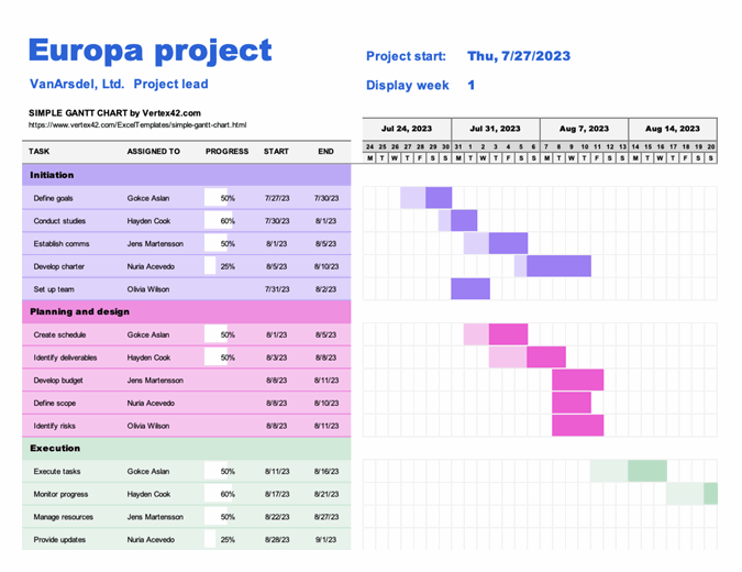The waterfall management style gets it’s name from the fact that work items are completed in a linear fashion with a cascading dependency chart such as that above.

With a agile mindset the main focus is on outcomes and deliverables, with the design and execution and delivery occurring in cycles. An agile approach works well in situations where the path to completion is not well defined, or where resources or requirements are liable to change throughout the project. Without knowing it you will probably already be engaged in a very agile-like approach to your research projects simply because so much of your work is likely to be exploratory in nature.


In a research context, an agile approach is all about exploring and responding to change (discoveries). You don’t know the outcome of your work before you start.

A common tool for visualizing and tracking work, particularly in an agile process, is the kanban board. The Kanban board was initially as a physical pin board on which cards or sticky notes were used to represent tasks. The tasks are organized into columns based on their status, and would typically migrate left to right across the board. Columns are customized for each project, but there are typically no more than 4-5. If a board is tracking multiple projects, or a project has multiple deliverables, then the board can also be divided horizontally into swimlanes. As the name suggests, tasks can move within a swimlanes, but are not intended to change lanes.


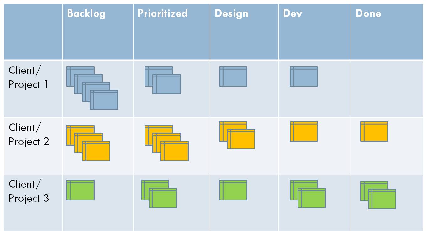An example of a Kanban board with 5 columns and 3 swimlanes

Design a board

Think of a project that you are currently working on and design a Kanban board for it. Consider the following:

How many task status categories are needed and what do you label them.

Could you get away with fewer categories?

Would it be useful to divide your tasks into different swimlanes, and if so how?

What tasks could you put in each category right now?

Using a simple markdown format create a table in our shared document that shows the categories (and swimlanes if used) that you would use for your project. If you have time include some example tasks. (See the example table).

Online Kanban with Trello

Trello is one of the most popular project management applications thanks to it being easy to use, flexible, and free.

If you have not already, create a Trello account here.

Trello organizes your tasks by workspaces and boards. Tasks that relate to a project are grouped into the same boards, and then multiple related boards are grouped into a workspace. For example you may have a different board for each of your research projects, but then group them together based on your collaborations. If you are doing a PhD then you’ll probably just need a single board for your PhD, and a single workspace to hold that board. As an early career researcher you’ll probably have a workspace that is something like “my astro work”, which then has a different board for each of the projects that you are involved in. Many people find it useful to also have a “personal” or “home life” board that they use to track non-work related activities. These are good people.

Trello uses a Kanban board to track tasks for each of your boards, and this is the default visualization that you’ll see when you create a board. The different columns within a board are referred to as “lists” and items within the list are “cards”. You will have the freedom to create/rename/delete the lists as you see fit, and to move cards between lists as they move through the to-do/doing/done phases that you define.

Cards have a lot of features that you can play with. Some of the immediately useful ones include:

a due date
embedded check lists for incremental tasks
customizable coloured labels
attachments
The ability to use markdown to format the text of the card
A chat/discussion space


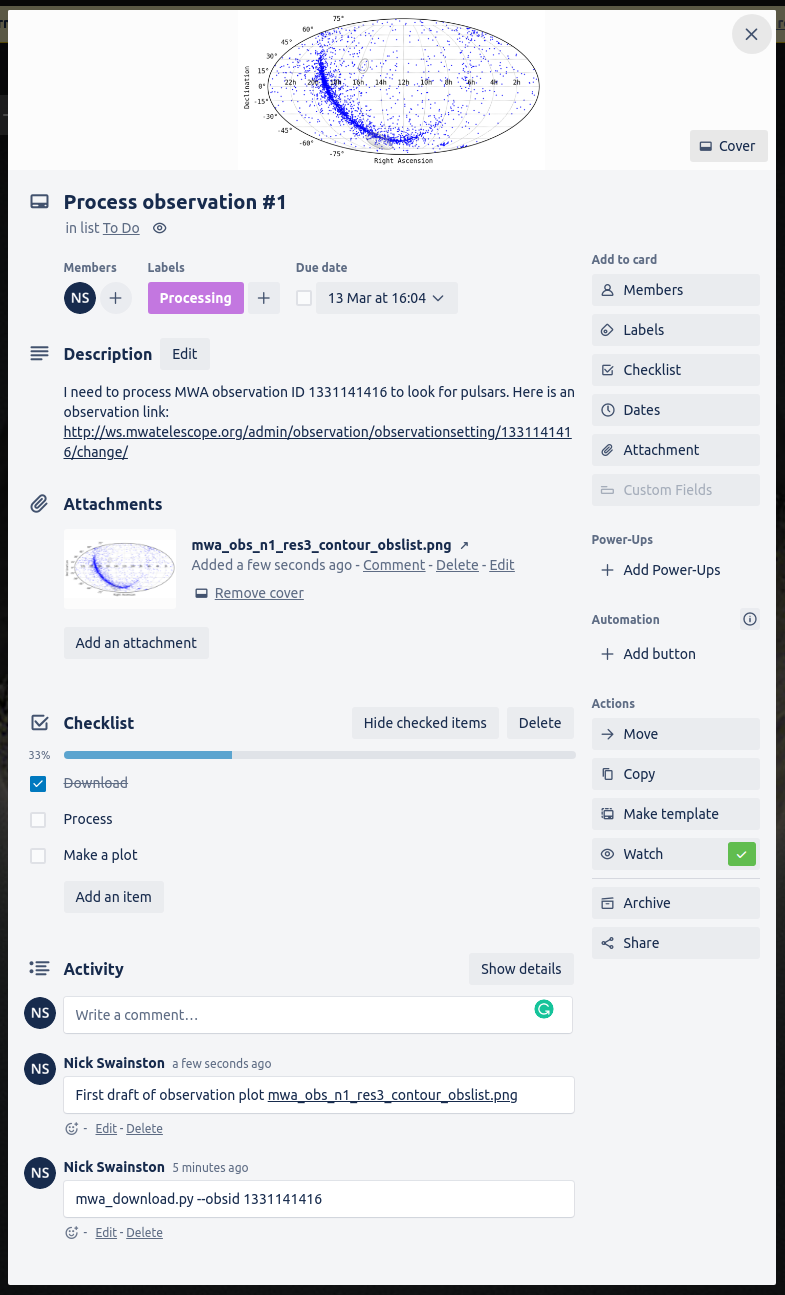An example of some of the features that you can add to your cards

Now that we have that nomenclature out of the way, lets get started with our Trello accounts.

Create a board with some dummy cards

Create a new workspace

Within that workspace create a new board

Within that board create three columns “todo”, “doing”, and “done”

Within the “todo” column create a new card

Set the title of the card to be something like “Create a card”

Move the card into the “doing” column

Add yourself as a member of the card

Add a short description to the card

Move the card to the “done” column

Pat yourself on the back for a job well done.

Time management

Part of managing a project is realizing that time is a very limited resource so it is often beneficial to manage it to the best of your abilities. You can split time management into two main catagories, prospective (planning) and retrospective (tracking).

A common way of estimating time projects will take is to work in hours/days/weeks/months of effort. However you are often not working on a single task at a time so it can be easier to break your total time available (your Full-Time Equivalent or FTE), into fractions, and then assign these fractions to different tasks. By estimating and tracking your FTE over the course of a project you can ensure that you are not spread too thin and you can finish tasks on time. Effective time management will prevent you from taking on more work than you can realistically complete.

For example, someone asks you to help with a project. You look at your project planning app and see that you have two projects you aim to spend 0.4 FTE on and a third you aim to spend 0.2 FTE on. Since this fills up the entire 1.0 FTE, you let them know that you can not assist on their project. You know that your third project will be complete in a month, so you offer to provide help at the level of 0.2 FTE starting in a month.

Deciding where you spend your FTE is only half the battle. You must also track your time to ensure that you are staying on budget, and adjusting if required. Tracking your time can be done through several apps (see the following section) and should give you at least a rough estimate of the time you spend on each project. This basic information will allow you to see how much time tasks and projects take and improve your future estimates. For example, you estimated that it would take you a month to write the first chapter of your thesis, but it took six weeks. You now know to budget more time for the next chapter. Another example is that you budget 0.5 FTE for teaching, but you realize you are using 0.6 FTE, so you will have to cut back on other projects.

How to track your time

There is a large variety of time tracking techniques and software available to help you track your time. Probably the most useful for academic work is an online or mobile app. Some time tracking apps are feature rich with all kinds of integrations and billing options, however they can come with a large time overhead which can be counter productive. If you are spending more than 10 minutes per day tracking your time, it is unlikely to be worth the effort, so we will focus on simple time tracking methods.

Excel method

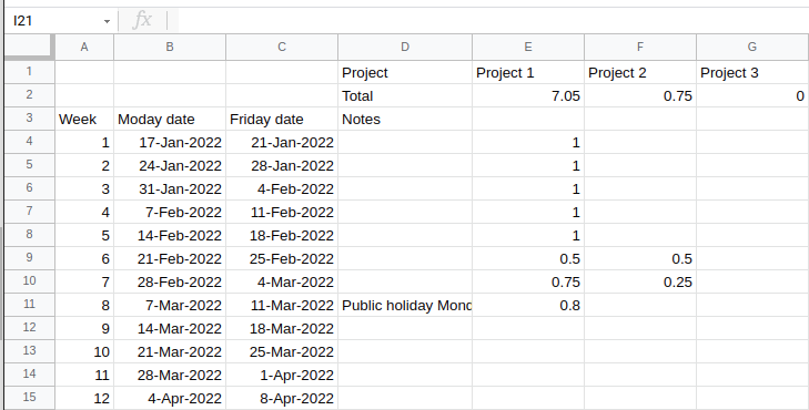
Here is a link to a simple Google Sheets template (shown below) of an easy way to track how much time you spend per week on several projects. At the end of each week, you update the sheet to track the fraction of your time you spent on each project. Additional projects can be added easily as new columns. This is effective for when you only care about your fractional FTE at a fairly low resolution. excel_method

Chronos app

Chronos is a simple app that will allow you to keep track of your project time. Simply make a new project with a descriptive name and set the billing type to non-billable. You can start a timer for the project you are currently working on or manually add how many hours you have spent. This method is good for when you have many projects that you are swapping between throughout the day, or when you want to be able to track your ‘effective’ work hours within a week. chronos_example

How do you spend your time?

Think about the work that you do as part of your research.

Itemize the projects/work that you do (up to 10 max)

For each item how much time you want to spend on it

For each item estimate how much you think you spend on it

Use our shared document to comment on why these last two might be different

Consider:

Of the three methods described for time tracking which would be more useful to you

“Owning” your project

Your PhD and research career is a story in progress and you are the hero protagonist. As with any good story, the hero goes through an arc of personal development. For you, this will likely be a progression from being led by your supervisor in a project that they conceived to being the expert in an area and being the main driver of your research. You will likely start out turning up to meetings that your supervisor calls, doing what you are told, reading all the suggested readings, and relying on your supervisor for the “next steps”. Eventually you will turn up to meetings that you organize, deciding on what your project goals are and how you’ll progress toward them, and handing out todo items at the end of a meeting. This is what we call “owning” your project, and when it happens you’ll feel less like an imposter, and more in control of your work (and life!). When your supervisor or mentor sees this transition is also very rewarding for them!

Much of the above will come naturally with time, but there are things that you can start thinking about now that will help you own your project now. Some key owning behaviors include:

Setting clear expectations for what work needs to be done, including deadlines
- Let people know how much time you have to work on something and when you expect it to be complete
Clear communication on progress, including any risks or slippages
- Let people know when you complete tasks or if there are road blocks
Taking the lead on project ideas
- You don’t have to have all the solutions, but making suggestions and asking the right questions is extremely helpful to everyone
Having meeting agendas and showing up to meetings with all the information that you need
- Send plots/text ahead of time for review, have the relevant files/pages open on your laptop ready to share

Discussion - how do/will you own your project

Think about the relationship you have with your group/supervisor

Identify an owning behavior that you are already doing

Identify an issue that you have and would like some advice with

Identify something that you are currently doing that has avoided some of the problems that we started the lesson with link

Share your ideas in our shared document

Key Points

Project and time management is key to success

Many tools exist, find one that works for you and stick with it

You PhD project is your’s for the taking

Bonus Content

Overview

Teaching: 0 min
Exercises: 0 min

Questions

What else is there?

Objectives

review some content that was too important to skip but didn’t fit in our lessons

Bonus Content

Bash as a scripting language

Bash is far more than a terminal, it’s a whole language in it’s own right. What we use as our terminal is equivalent to the interpreter we interact with when we type python3 on the command line. A few key things to know about bash to get you started are:

variables can be set like fname=myfile.csv (with no spaces around the =)
variables can be accessed using ${fname} or the slightly more relaxed $fname
A file that starts with #! /usr/bin/env bash and has execute permissions (chmod +x <filename>) can be run directly
flow control uses if ... then ... else .. fi syntax
new line continuation is accomplished by having \ as the last character on the line
converseley, multiple commands can be used on a line, separate them with ;
program output can be redirected to a file with > (replace) or >> (append)

For more info see this wikibook for a nice intro.

Depending on the task you are trying to accomplish, a bash script can be easier to work with than a python script.

Automation with aliases

A basic form of automation is the use of aliases. The goal here is to save you a bunch of keyboard or mouse clicks. Some common examples:

# long list all files
alias ll='ls -al'

# open ds9 and press about 20 buttons to get the interface set up just the way I like
alias ds9='~/Software/ds9/ds9 -scalelims -0.2 1 -tile -cmap cubehelix0 -lock frame wcs -lock scale yes -lock colorbar yes -lock crosshair wcs'

# run stilts and topcat and not have to bother with the java invocation
alias stilts='java -jar ~/Software/topcat/topcat-full.jar -stilts'
alias topcat='java -jar ~/Software/topcat/topcat-full.jar'

# activate my favorite python3 environment
alias py3='source ~/.py3/bin/activate'

Structured data storage

CSV files are great but can be cumbersome to work with when they become large or when you have multiple files with related data. An alternative is to store your data as tables in a database, where you can make explicit links between multiple tables, and make use of the SQL language to select, filter, order, and extract the data that you need. Some commercial (but free) solutions include PostgreSQL and MySQL, but these require a fair bit of system admin to get setup and work with. A great lightweight middle-ground is SQLite, which provides the core functionality of a relational database but without all the security, authentication, and sys admin requirements of a commercial solution. See this carpentries lesson for an introduction do databases using SQLite.

Task prioritization

In most cases you will have more tasks than time available to do said tasks. You will therefore need some way of determining which tasks should be done and which can be left undone or done at a later time. A common metric to decide on the order to do tasks is the priority matrix:

PriorityMatrix

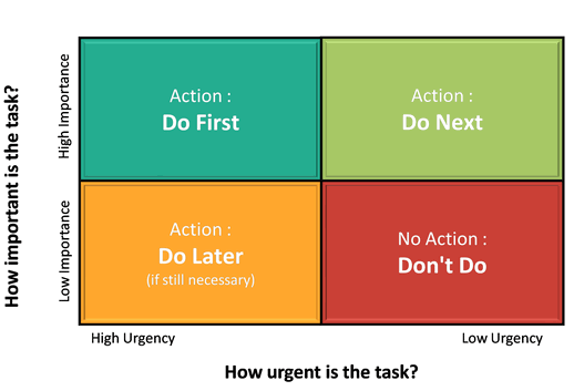
You can incorporate the above priority matrix into your work planning in a number of ways:

Use these four categories as columns in your kanban board
Create labels with corresponding name/colour to add to each of the tasks in your kanban board
Create swimlanes for your kanban board that correspond to these categories (though tasks may need to change lanes!)

An alternative priority matrix which could be useful for research work is one where you consider impact (research output) and effort (time to complete). This is useful when considering which projects to take on and their goals. Successful researchers are often skilled at identifying projects that are high impact with minimal effort.

Key Points

there is always more to learn

Skills for (academic) Life

Introduction and setup

Overview

Acknowledgement of country

Schedule

Content

Engagement

Conduct

Introduce yourselves

Key Points

Scientific Computing

Overview

Scientific Computing

Your computing journey

Automate your way to success

Your day-to-day sciencing workflow

Challenge

Solution notes

Favorite tools

Reproducible research

Discussion

Key Points

Morning Tea

Overview

Key Points

Best Practices In Scientific Computing

Overview

Best Practices In Scientific Computing

Use case - visualizing a data set

output

output

Start a new project

Save your progress

output

Save your progress

Delete some code and check it in

Pre-existing solutions

Visualizing data

Our first plot

Save your progress

Our second plot

Save your progress

Creating a reusable script

Let’s focus on New Zealand

Making your script re-usable

add a command line interface

Testing

Create test file

Documentation

Create a README file for your repo

Key Points

Lunch

Overview

Key Points

Managing Data

Overview

Managing Data

Types of data

Discussion

Structured data

Unstructured data

Exercise

Data cleaning

View the raw data

Solution with pandas

solution with bash

Challenge

Data storage and access

Structured data

Using SQL to select data

Challenge

Solution

Unstructured data

Meta-data

Key Points

Afternoon Tea

Overview

Key Points

Project Management

Overview