Overview

Teaching: 30 min
Exercises: 30 min

Questions

• Why do I need to manage data?

• How do I manage different types of data?

• How do I store and access structured data?

• How do I store and access unstructured data?

Objectives

• Distinguish between different types of data

• Understand how to work with structured and unstructured data

• Be comfortable with SQL select and filter queries

• Understand what meta-data is

Managing Data

All of our research is fundamentally reliant on data so it’s important to understand the different types of data, how to store them, and how to work with them. In this lesson we’ll learn all the above!

Types of data

Fundamentally computers store data as 0s and 1s, representing floats, integers, boolean, or character data types. However this is not what we are going to talk about here. Here we are more concerned with a higher level of abstraction, which includes the following data types:

• raw data
  • as it comes directly from a sensor or data source
  • contains signal + noise
  • format and quality is highly dependent on the data source
• clean data
  • has bad/invalid records removed or flagged
  • has been converted to a format which is usable by your analysis or processing tools
• transformed data
  • useful features have been identified
  • low level aggregation has been applied
  • instrument/sensor/model dependent effects have been removed
• reduced data
  • has been modeled
  • has been processed into a different form such as images or a time series
• published data
  • the highest level of abstraction/aggregation of your data
  • often represented as tables or figures

The following describes a generic data processing workflow

Discussion

In your groups have a look at the different types of data and stages of the data processing workflow. Think about:

• Where do you get your data from?
  • Are there more than one source of data?
• How do you keep track of which data is in which stage of processing?
• When you publish your work, which data products do you want to keep and which can be deleted?

Record some notes in the shared document.

We can classify data by the processing stage as was done above, but also in an orthogonal dimension of how the data is organized. The two most general considerations here are either structured or unstructured data.

The way that we can store and access data depends on how it’s structured.

Structured data

One of the easiest ways to store structured data are in one or more tables. The tables themselves can be stored as .csv, .fits, or .vot tables which can be read by many astronomy software tools such as topcat. Google sheets, Microsoft Excel, or LibreOffice Calc can also be beneficial for storing structured data, particularly because they allow you to do some data exploration, cleaning, filtering, and analysis within the file itself.

When your data volumes become large, or you find yourself needing to have multiple related tables, then you probably want to start exploring databases as a storage option. See the Bonus Content

Unstructured data

Unstructured data cannot be aggregated or combined into a single data format due to their lack of common structure. In such cases it is often best to make use of a regular directory/file structure to store the individual files in a way that can be navigated easily. A well planned directory/file structure it is very useful to store meta-data about each of the files that you are storing. For example you could have:

• A README.md file in the root directory that describes the directory/file structure
• A metadata.csv file that maps the location of a file to some high level information such as the file format, the date the file was collected, the processing stage of the data, or the version of the file.

Exercise

• Download example data example.zip
• Unzip the file and have a look at the content
• See if you can infer the purpose of each file
• Make a plan for how you would store and manage this data
• Note in the shared document what you have decided for at least one of the files

Data cleaning

In the previous lesson we worked with a file Australian_Meteorite_Landings.csv. For your benefit this had already been cleaned to remove invalid entries, attributes that we didn’t need, and entries that were not relevant.

Let’s now start with the original data set and go through the cleaning process.

wget -O Meteorite_Landings.csv https://data.nasa.gov/api/views/gh4g-9sfh/rows.csv?accessType=DOWNLOAD
# or
curl -o Meteorite_Landings.csv -O https://data.nasa.gov/api/views/gh4g-9sfh/rows.csv?accessType=DOWNLOAD

Now we’ll explore the data set using pandas.

View the raw data

Using your viewer of choice, have a look at the csv file that we just downloaded. Think about and discuss:

• Are there any missing data?
• What can be done about the missing data?
• Are there any columns that are not useful?

Note in our shared document which tool you used to inspect the data, and one that you would take to clean this data.

Solution with pandas

import pandas as pd
df = pd.read_csv('Meteorite_Landings.csv')
print("Quick look of data")
print(df)
print("Summary of data")
print(df.describe())

Quick look of data
             name     id nametype              recclass  mass (g)   fall    year    > reclat    reclong             GeoLocation
0          Aachen      1    Valid                    L5      21.0   Fell  1880.0  50.> 77500    6.08333       (50.775, 6.08333)
1          Aarhus      2    Valid                    H6     720.0   Fell  1951.0  56.> 18333   10.23333    (56.18333, 10.23333)
2            Abee      6    Valid                   EH4  107000.0   Fell  1952.0  54.> 21667 -113.00000      (54.21667, -113.0)
3        Acapulco     10    Valid           Acapulcoite    1914.0   Fell  1976.0  16.> 88333  -99.90000       (16.88333, -99.9)
4         Achiras    370    Valid                    L6     780.0   Fell  1902.0 -33.> 16667  -64.95000     (-33.16667, -64.95)
...           ...    ...      ...                   ...       ...    ...     ...       ..> .        ...                     ...
45711  Zillah 002  31356    Valid               Eucrite     172.0  Found  1990.0  29.> 03700   17.01850       (29.037, 17.0185)
45712      Zinder  30409    Valid  Pallasite, ungrouped      46.0  Found  1999.0  13.> 78333    8.96667     (13.78333, 8.96667)
45713        Zlin  30410    Valid                    H4       3.3  Found  1939.0  49.> 25000   17.66667       (49.25, 17.66667)
45714   Zubkovsky  31357    Valid                    L6    2167.0  Found  2003.0  49.> 78917   41.50460     (49.78917, 41.5046)
45715  Zulu Queen  30414    Valid                  L3.7     200.0  Found  1976.0  33.> 98333 -115.68333  (33.98333, -115.68333)

[45716 rows x 10 columns]
Summary of data
                 id      mass (g)          year        reclat       reclong
count  45716.000000  4.558500e+04  45425.000000  38401.000000  38401.000000
mean   26889.735104  1.327808e+04   1991.828817    -39.122580     61.074319
std    16860.683030  5.749889e+05     25.052766     46.378511     80.647298
min        1.000000  0.000000e+00    860.000000    -87.366670   -165.433330
25%    12688.750000  7.200000e+00   1987.000000    -76.714240      0.000000
50%    24261.500000  3.260000e+01   1998.000000    -71.500000     35.666670
75%    40656.750000  2.026000e+02   2003.000000      0.000000    157.166670
max    57458.000000  6.000000e+07   2101.000000     81.166670    354.473330

solution with bash

head Meteorite_Landings.csv

name,id,nametype,recclass,mass (g),fall,year,reclat,reclong,GeoLocation
Aachen,1,Valid,L5,21,Fell,1880,50.775000,6.083330,"(50.775, 6.08333)"
Aarhus,2,Valid,H6,720,Fell,1951,56.183330,10.233330,"(56.18333, 10.23333)"
Abee,6,Valid,EH4,107000,Fell,1952,54.216670,-113.000000,"(54.21667, -113.0)"
Acapulco,10,Valid,Acapulcoite,1914,Fell,1976,16.883330,-99.900000,"(16.88333, -99.9)"
Achiras,370,Valid,L6,780,Fell,1902,-33.166670,-64.950000,"(-33.16667, -64.95)"
Adhi Kot,379,Valid,EH4,4239,Fell,1919,32.100000,71.800000,"(32.1, 71.8)"
Adzhi-Bogdo (stone),390,Valid,LL3-6,910,Fell,1949,44.833330,95.166670,"(44.83333, 95.> 16667)"
Agen,392,Valid,H5,30000,Fell,1814,44.216670,0.616670,"(44.21667, 0.61667)"
Aguada,398,Valid,L6,1620,Fell,1930,-31.600000,-65.233330,"(-31.6, -65.23333)"

wc Meteorite_Landings.csv

  45717  166894 3952161 Meteorite_Landings.csv

You may have noticed when inspecting the file above, that the header names are occasionally useful, but don’t do a good job of explaining what the data represent. For example:

• what does the “rec” in reclat/reclong represent?
• Why do some meteors have blank reclat/reclon, while others have (0,0)?
  • Did someone found a meteorite at the Greenwich observatory?
• There are many meteorites with the same reclat/reclong, why is this?
• What does recclass represent?

Here is where we need to think about the meta-data attached to this table. We need context (how/why the table was created), and also a description of what the data represent. If we go to the NASA website which provides this data, they have a description of the column data. However, it’s not so helpful:

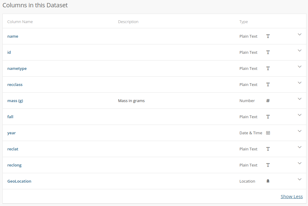
Wuh-wah! The only column with a description is the one that was most obvious. Not only that, but the data type listed for the columns is incorrect in many cases. For example, id, reclat, and reclat are listed as being “plain text” but they are clearly numeric (int, and floats), while “year” is listed as being “date and time”.

Enough complaining, lets start fixing.

Challenge

We want to plot all the Australian meteorites, with a measured mass value, and a nametype of “Valid”

• Using pandas, load the meteorite dataset
• Delete the geolocation column as it’s a duplicate of the reclat/reclong columns
• Select all rows with a non-zero and non-null mass value
  • Count the rows and record this number
  • Delete these rows
• Repeat the above for:
  • rows with a reclat/reclong that are identically 0,0
  • rows with a blank reclat/reclong
  • rows with nametype that is not “Valid”
• Delete the nametype column as it’s now just has a single value for all rows
• Choose a bounding box in lat/long for Australia (don’t forget Tassie!)
• Select, count, and delete all rows that are outside of this bounding box
• Save our new dataframe as a .csv file
• Run our previously created script on this file and view the results

Data storage and access

The way that you store and access data depends on many things including the type of data, the structure of the data, and the ways that you will access and use the data.

We’ll focus here on the two data types introduced at the start of this lesson: structured and unstructured data.

Structured data

These are the kinds of data that we can store as rows in a .csv file or Excel spreadsheet. The two options for storing these data would be flat files or a database. A flat-file is, as the name suggests, a single file which contains all the information that you are storing. You need an independent program to load/sort/update the data that is stored in a flat-file. As the data volume becomes large, or the relation between data in different flat-files becomes more intertwined the creation, retrieval and management of these files can become time consuming and unreliable.

A database is a solution that combines the data storage, retrieval, and management in one program. A database can allow you to separate the way that the data are stored logically (tables and relations) and physically (on disks, over a network).

We’ll explore some basics of data bases using sqlite3. This program supports the core functionality of a relational database without features such as authentication, concurrent access, or scalability. For more advanced features you can use more full featured solutions such as PostgreSQL or MySQL. One of the nice things about sqlite3 is that it stores all the data in a single file, which can be easily shared or backed up. For this lesson we’ll be working with a ready made database Meteorite_Landings.db.

Using SQL to select data

There are two choices of how you can use sqlite3 for this lesson:

1. run sqlite3 Meteorite_Landings.db from your terminal
2. Go to sqliteonline.com and upload the file

The data in a database is stored in one or more tables, each with rows and columns. To view the structure of a table we can use:

.schema

CREATE TABLE IF NOT EXISTS "landings" (
"index" INTEGER,
  "name" TEXT,
  "id" INTEGER,
  "nametype" TEXT,
  "recclass" TEXT,
  "fall" TEXT,
  "year" REAL,
  "reclat" REAL,
  "reclong" REAL,
  "GeoLocation" TEXT,
  "States" REAL,
  "Counties" REAL,
  "mass" REAL
);

What we see in the output here are the instructions on how the table was created. The name of the table is landings, and there are a bunch of column names which we recognize from previous work. We can see that each column has a particular data type (TEXT, INTEGER, REAL). In a database the types of data that can be stored in a given column are fixed and strictly enforced. If you tried to add “one” to a column with type REAL, then the database software would reject your command and not change the table.

If we want to see the content of the table, we need to SELECT some data. In SQL we can do this using the SELECT command as follows:

SELECT <columns> FROM <table>;
SELECT name, mass, year FROM landings;
SELECT * FROM landings;

The last command is the most common command for just looking at the table content as it will show all the columns without you having to list them all. If we want to show only the first 10 lines (like head) then we can choose a LIMIT of lines using:

SELECT * FROM landings LIMIT 10;

Note that if you are using the command line version of sqlite3 the default output can be a little hard to read. Firstly, you’ll get all the data speeding by. Secondly, the data are not well formatted for humans to read. We can fix this with a few commands:

.mode column
.headings on

Combining all this together we have the following:

sqlite> SELECT * FROM landings LIMIT 10;

index       name        id          nametype    recclass    fall        year        reclat      reclong     GeoLocation        States      Counties    mass      
----------  ----------  ----------  ----------  ----------  ----------  ----------  ----------  ----------  -----------------  ----------  ----------  ----------
0           Aachen      1           Valid       L5          Fell        1880.0      50.775      6.08333     (50.775, 6.08333)                          21.0      
1           Aarhus      2           Valid       H6          Fell        1951.0      56.18333    10.23333    (56.18333, 10.233                          720.0     
2           Abee        6           Valid       EH4         Fell        1952.0      54.21667    -113.0      (54.21667, -113.0                          107000.0  
3           Acapulco    10          Valid       Acapulcoit  Fell        1976.0      16.88333    -99.9       (16.88333, -99.9)                          1914.0    
4           Achiras     370         Valid       L6          Fell        1902.0      -33.16667   -64.95      (-33.16667, -64.9                          780.0     
5           Adhi Kot    379         Valid       EH4         Fell        1919.0      32.1        71.8        (32.1, 71.8)                               4239.0    
6           Adzhi-Bogd  390         Valid       LL3-6       Fell        1949.0      44.83333    95.16667    (44.83333, 95.166                          910.0     
7           Agen        392         Valid       H5          Fell        1814.0      44.21667    0.61667     (44.21667, 0.6166                          30000.0   
8           Aguada      398         Valid       L6          Fell        1930.0      -31.6       -65.23333   (-31.6, -65.23333                          1620.0    
9           Aguila Bla  417         Valid       L           Fell        1920.0      -30.86667   -64.55      (-30.86667, -64.5                          1440.0    

By convention we use all caps for the keywords, and lowercase for table/column names. This is by convention only, and sqlite3 is not case-sensitive.

We can filter the data that we retrieve by using the WHERE clause.

SELECT <columns> FROM <table> WHERE <condition> LIMIT 10;

Challenge

• Find all the meteorites that fell between 1980 and 1990, and have a mass between 100-1,000g.
• List the name and reclat/reclong for 15 of these meteorites

Solution

sqlite> SELECT name, reclat, reclong FROM landings WHERE year >= 1980 AND year <=1990 LIMIT 15;

name        reclat      reclong   
----------  ----------  ----------
Akyumak     39.91667    42.81667  
Aomori      40.81056    140.78556 
Bawku       11.08333    -0.18333  
Binningup   -33.15639   115.67639 
Burnwell    37.62194    -82.23722 
Ceniceros   26.46667    -105.23333
Chela       -3.66667    32.5      
Chiang Kha  17.9        101.63333 
Chisenga    -10.05944   33.395    
Claxton     32.1025     -81.87278 
Dahmani     35.61667    8.83333   
El Idrissi  34.41667    3.25      
Gashua      12.85       11.03333  
Glanerbrug  52.2        6.86667   
Guangnan    24.1        105.0     

You can interact with a database programmatically using the python module sqlite3. With the combination of sqlite3 and pandas modules, you can save a pandas data frame directly to a database file. This is one of the easiest ways to create a simple database file.

import sqlite3 as sql
import pandas as pd

# read the .csv file
df = pd.read_csv("Meteorite_Landings.csv")
# create a connection to our new (empty) database
con = sql.connect("Meteorite_Landings.db")

# update the name of mass column to avoid spaces and special chars
db['mass'] = db['mass (g)']
del db['mass (g)']

# save the dataframe to the database via the connection
df.to_sql(name='landings', con)

Unstructured data

Data that doesn’t conform to a standard tabular format are referred to as unstructured data. For example:

• images,
• videos,
• audio files,
• text documents

For these data we still need to be able to know where it is and where to put new data. In this case we can impose some structure using a directory/file structure. The structure that you use ultimately depends on how you’ll use the data.

For example, imagine that we have a photograph of each of the meteorites represented in our landings table from the previous exercise. The images could be organized in one of the following ways:

name.png
<name>/<location>/id.png
<continent>/<year>/id.png
<recclass>/<year>/name.png
<state>/<county>/<year>/<recclass>/id.png

In each of the above examples you can see that there is an intentional grouping and sub-grouping of the files which make sense for a given type of analysis, but will be confusing or tedious to work with for a different type of analysis. For example, <continent>/<year>/id.png will be convenient if you are looking at how meteorite monitoring/recovery has progressed in various countries over time, but it will be annoying to work with if you just want to select meteorites with a particular composition. Whatever choice you make for storing your data, it is a good idea to make a note of this scheme in a file like README.md or file_structure.txt, so that you and others can easily navigate it.

You could start to encode extra information into the filenames, and then describe this naming convention in the README.md file.

A very nice hybrid solution is to use a database to store some information about your image files in a table, and have a column which is the filename/location of the image file. In our example, this would mean appending a single new column to our existing database table or .csvfile. In the case where the data are the images, then you would need to start extracting information about the data (meta-data) from each of the files, and then store this in a database or table. For example if you have a set of video files you could extract the filming location (lat/long), time, duration, filename, and some keywords describing the content. This solution allows you to query a database to find the files that match some criteria, locate them on disk, and then use some video analysis software on each.

Meta-data

• Think about some of the unstructured data that you collect or create as part of your research work
• Write a short description of what these data are
• Choose 4-5 pieces of metadata that you would store about these data
• Use our shared document to share you description and meta-data

Key Points

• Invest time in cleaning and transforming your data

• Meta data gives context and makes your data easier to understand

• How and where you store your data is important