How to Accelerate your Research

Overview

Teaching: 45 min
Exercises: 45 min

Questions

• What are the benefits of scaling resources over optimizing code?

• How can multiple cores be utilized effectively?

Objectives

• Understand the concept of scaling resources to accelerate research.

• Learn how to use multiple cores in parallel computing.

• Identify and address common research bottlenecks.

Overview

When you have offloaded much of your work to a computer your productivity becomes limited by computing resources. A common misconception is that faster code requires a deep dive into the world of code optimization. This is, however, just a misconception: there are many ways to speed up your research that don’t require you to rewrite your code at all (or much).

Today’s focus

Today we will consider an example task that is integral to our research work, but is taking a long time to complete. The completion of this task is a bottleneck for progress. We will look at how to make use of more resources on our own computer in multiple different ways, and then talk about what it takes to use HPC resources.

Example workflow

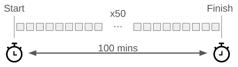
Suppose that we have a workflow that is composed of some number of sub-tasks. In the simplest case, this workflow isn’t really a “flow” - it’s just a list of things to do that don’t depend on each other. For argument sake, lets assume there are 50 tasks, each taking 2 mins to complete, so that the user has to wait 100 minutes between starting the workflow, and seeing it completed.

In general you have the following options available to you:

1. Do nothing.
   • Accept that the time taken is unchangeable and just make do.
   • This requires zero investment of time, and is a good option if you never plan to run the workflow more than once.
2. Make the individual tasks take less time:
   • Optimize the code to be more efficient (typically large time investment)
   • Run the same code on faster hardware (typically small time investment)
3. Do multiple tasks at once:
   • Run one task per cpu available (being aware of RAM limits)
   • Run your workflow on multiple computers at once (desktops, or nodes of an HPC)
4. Skip some of the tasks:
   • Save the outputs of each task, and only re-run them as needed (checkpointing or caching)
   • Caching is a typical space-time tradeoff but is also one of the Two hard problems in computing

We are going to not engage in 1 because there is nothing to teach. We will not explore 4 except to say that make and NextFlow both have a caching mechanism that you can use without having to write any extra code. The focus of today’s workshop will be on 2 and 3 - making things faster and doing more work at once.

Planning your workflow for speed

When you are building a workflow you should firstly determine what tasks are needed to get to your goal. If some of these tasks involve multiple steps, consider breaking them into a sub-workflow of smaller tasks For each of the tasks that you need to complete, determine what input data/information is required, and what outputs they produce. Join all your tasks together into a flow chart such as the one below, taken from Hancock et al. 2019.

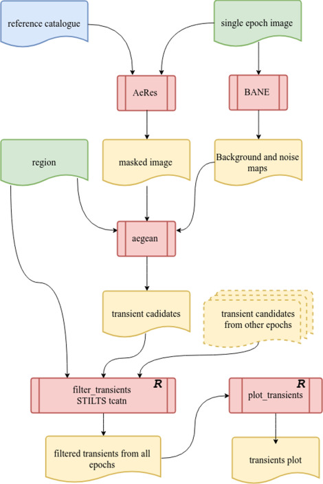
In the above diagram we have red boxes representing work to be done, while the green and yellow boxes show data that is required/produced by each step. Note the yellow dashed box labeled “transient candidates from other epochs”. This represents the fact that the upper part of this diagram is done repeatedly for multiple different images/epoch, and is then combined together for the final two red boxes. This is a way of identifying what components can be done in parallel.

Some common patterns that you will see in workflows are:

• one-to-one
  • A single task produces output that is consumed by another task
• many-to-one
  • Multiple tasks produce output, which together are all required for the next task
• one-to-many
  • One task produces multiple outputs, each of which are consumed by a single task
• one-to-many-to-one
  • A combination of the above, where the tasks in the “many” section are independent of each other.
  • These are excellent opportunities for parallelizing part of your workflow.
• many-to-one-to-many
  • The inverse of the above, where as single task requires many inputs and produces many outputs.
  • This can be a sign of a bottle-neck in your workflow.

Once you have determined which parts of your workflow could be run in parallel, and before you have done work to parallelize it, you should consider the return on investment. If you know how long each task will take, you can compute the fraction of tasks that have to be run in series and the fraction that can be run in parallel. Amdahl’s law gives you an estimate (upper limit) of the speed up factor.

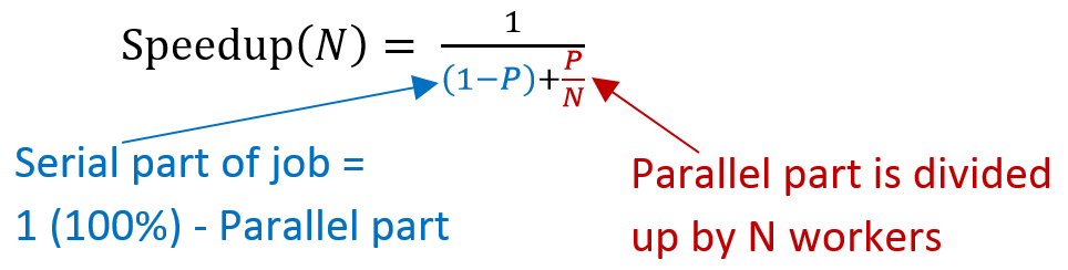
In general you won’t achieve this factor, because there are always overheads associated with parallel execution (such as communication, or resource contention), but it is often not hard to come close to this factor. Therefore, you should think about wether it’s worth investing the time.

Making things go faster

When thinking about the problem, remember that your code doesn’t run in isolation. It runs as part of a larger workflow, that includes other pieces of code as well as non-automated things like researcher thinking time. Consider your entire workflow, and how much time is spent on waiting for code to run vs you analyzing results. If you have other useful work that can be done while your code runs, then do that, it’ll be time well spent.

Amdahl’s Law:

• System speed-up limited by the slowest component.

Paul’s rule of thumb:

• You are the slowest component.

Therefore:

1. Focus on reducing your active interaction time, (automation)
2. then on your total wait time, (using more resources)
3. then on cpu time (optimization).

A reason to confirm that we need to optimize our code is that we want to avoid premature optimization:

Writing performant code

Code optimization is the process of improving the efficiency of your code to reduce execution time, memory usage, or other resource consumption. However, optimization should be approached carefully to avoid unnecessary complexity or premature efforts. Below are key considerations and strategies for optimizing code (for speed):

1. When to Optimize
   • Measure First: Use profiling tools (e.g., cProfile, line_profiler) to identify bottlenecks in your code.
   • Set Goals: Define what “good enough” performance looks like for your use case.
   • Avoid Premature Optimization: Focus on correctness and clarity first; optimize only when necessary.
2. General Strategies
   • Use Efficient Algorithms: Choose algorithms with better time and space complexity for your problem.
   • Leverage Existing Libraries: Libraries like numpy, pandas, and scipy are highly optimized for performance.
   • Minimize Redundant Computations: Cache results of expensive operations if they are reused (e.g., memoization).
3. Python-Specific Tips
   • Vectorization: Replace loops with vectorized operations using libraries like numpy.
   • Data Structures: Use appropriate data structures (e.g., set for membership checks, deque for queues).
   • Avoid Global Variables: Accessing global variables can slow down your code due to namespace lookups.
4. Iterative Optimization
   • Test After Each Change: Ensure that optimizations do not introduce bugs or regressions.
   • Benchmark: Use tools like timeit to measure the impact of your changes.

In this workshop we aren’t going to do any optimization, for that you can check out our other lessons here or here. Instead, we will talk about how you can write code that is likely be to be “pretty fast” or “good enough” to start with - performant code.

Don’t repeat others

The first thing to note is that other people have been writing code for a lot longer than you have and there are some true experts out there that spend a lot of time making their code as fast as possible. Rather than trying to compete with them, or reproduce their efforts, you should look to build upon their success. So before you start to code up some functions, workflows, or libraries, have a look online and see if you can find some existing libraries. Some excellent examples that most people likely already use are numpy, scipy, pandas, and astropy. These libraries are developed by teams of folks who pay close attention to getting the right answer, in the shortest time possible, and usually without exploding your RAM.

Places to look for useful libraries:

• Your peers and collaborators - ask what other people are using (bonus, they also be a good source of help when things go bad),
• PyPI (Python Package Index) - the go-to source for Python packages (both good and bad),
• GitHub, as above, but not specific to python, probably a large fraction of not-great things,
• The acknowledgements section of papers you read - some kind souls mention/cite their code.

What are some of your go-to libraries?

Let us know an not-yet mentioned library that you often use in your work. Give a 1 sentence description of what the library is designed for.

Use the collaborative notes or the zoom chat to share.

Using existing libraries means that you’ll be importing functions, but also data structures. It is good practice to use the recommended data structures with the given library functions as this reduces the amount of type casting and conversion work that needs to be done. Let’s explore how this would work using an example from numpy.

For a basic example we’ll consider performing an operation on two sets of data. Supposed we have two lists of integers (A and B), and we want to add them together (C = A + B).

Add two python lists

Using ipython do the following and observe the output:

A_list=list(range(10_000))
B_list=list(range(10_000))

%timeit C_list = [ a+b for a,b in zip(A_list,B_list)]

Output

Depending on the speed of your computer you’ll get something like this:

295 μs ± 26.5 μs per loop (mean ± std. dev. of 7 runs, 1,000 loops each)

Now let us use the numpy data types. These are numpy arrays rather than python lists.

Add two numpy arrays

Again using ipython, do the following and observe the output:

# assuming the same session as before
import numpy as np
A = np.array(A_list)
B = np.array(B_list)
%timeit C = A+B

Output

Depending on the speed of your computer you’ll get something like this:

2.01 μs ± 71.7 ns per loop (mean ± std. dev. of 7 runs, 100,000 loops each)

So we have a speed up of about 100x (for that one operation), just by using numpy data types and leveraging the fast algebra that numpy provides. numpy contains more than just basic math functions. In fact many of the linear algebra operations that you would want to perform on arrays, vectors, or matrices (in the numpy.linalg module), call on powerful system level libraries such as OpenBLAS, MKL, and ATLAS. These libraries, in turn, are multi-threaded or multi-core enabled, so in many cases you’ll also be able to make use of multiple cores, without having to explicitly deal with the multiprocessing library, just by using numpy or scipy functions. Some particularly useful examples are the scipy.optimize and scipy.fft modules.

Other examples of this vectorized approach include:

• scipy
  • Because it’s a wrapper around numpy in many cases.
• pandas
  • Operations on columns are vectorized.
• astropy
  • Instead of an array of SkyCoord objects, create a single SkyCoord with arrays of coordinates. Operations on this object will be vectorized.
  • With two SkyCoord objects (catalogues) you can run a cross-match between them. Astropy will do the matching using an algorithm much smarter than your “minimum of the all to all comparison”.

The main lesson here is that Python is slow but easy to code, and C is fast but hard(er) to code, but by using libraries such as numpy you can start to get the benefit of both worlds - easy to code, fast to use. So, wherever possible, use already built libraries and avoid re-implementing things yourself.

Scaling Up Your Resources

Using faster hardware

In the 1980s and 1990s, the performance of computers improved significantly due to increasing CPU clock speeds. Manufacturers were able to make processors faster by shrinking transistor sizes and improving fabrication techniques. This trend, often referred to as “Moore’s Law,” led to a doubling of transistor density approximately every two years, which translated into faster CPUs. Buying a new computer usually meant you were buying a faster CPU so your programs would run faster.

However, around the early 2000s, this trend began to slow down. Increasing clock speeds further became challenging due to physical limitations such as heat dissipation and power consumption. As a result, the focus shifted from making individual cores faster to adding more cores to processors. This marked the beginning of the multi-core era.

Modern CPUs now often have multiple cores, allowing them to perform many tasks simultaneously. While individual cores may not be significantly faster than those from the early 2000s, the ability to run multiple processes in parallel has led to substantial performance improvements for workloads that can take advantage of parallelism. This shift has made understanding and utilizing parallel computing essential for researchers and developers. Unless you are using a truly ancient piece of hardware, buying a “faster” computer isn’t going to make your single CPU task take less time to run. In fact, a new desktop computer may have 5GHz clock speed, where as an HPC facility may have CPUs with only a 2.5GHz clock speed, so running your single core job on an HPC may actually take longer. (This is because HPC facilities provide many more CPU cores than your desktop: 64-128 vs 8-16).

However, if your task is running slow because it is being limited by disk read/writes, then swapping a spinning disk HDD for a SSD or nVME can make this go faster. Similarly if your task is running slow because it uses all your RAM, and has to start using disk storage instead (swapping or paging), then expanding the RAM could make things faster. This is where HPC really start to shine, because they often provide large amount of RAM per compute node, and will have various storage solutions that are optimized for read/write speed or for long term storage.

Using more cores

Most programs that you write will be executed on a single CPU core. Some python libraries (like numpy) will use system libraries that can use multiple CPUs, but only for some operations. While it can be difficult or impossible to rewrite your tasks to make use of multiple CPU cores at once, there is a much simpler option available to us if we look at the level of a workflow. The solution is to simply run different tasks on different cores.

If we have even a modest desktop computer we could have 8 cores available to us. If we were to divide our workflow among these 8 cores we could reduce the total execution time from 100 minutes, down to just 12.5 minutes. The exact same calculations are being done (e.g. there is no optimization), but because we have deployed 8x as much resources, we can get the job done in 1/8th of the time. This is what we call task based parallelism.

A high level approach to using multiple cores is the controller/worker approach. The controller/worker approach is a method of organizing scripts to enable modularity and reusability, which is particularly useful for parallel workflows. Here’s how it works and why it’s beneficial:

1. Controller Script
   • The controller script orchestrates the workflow.
   • It defines the overall logic, such as which tasks to execute, in what order, and how to distribute them across available resources (e.g., CPU cores or nodes).
   • Tools like xargs, GNU parallel, or job schedulers (e.g., SLURM) are often used in the controller script to manage parallel execution.
2. Worker Script
   • The worker script contains reusable functions or commands that perform specific tasks.
   • These tasks are modular and can be called by the controller script as needed.
   • The worker script is designed to handle individual units of work, such as processing a single file or performing a single computation.
   • The worker script can be written in any language, so long as it has a command line interface that the controller script can call.

How It Works in Parallel Workflows

1. Task Definition:
   • The worker script defines the task to be performed (e.g., processing a dataset, running a simulation, or generating a report).
   • Each task is self-contained and can be executed independently.
2. Task Distribution:
   • The controller script reads a list of tasks (e.g., from a file or generated dynamically) and distributes them across available resources.
   • Tools like xargs or GNU parallel are used to execute multiple instances of the worker script in parallel.
3. Parallel Execution:
   • Each instance of the worker script runs on a separate core or node, processing its assigned task.
   • The controller script ensures that tasks are executed efficiently, respecting resource limits (e.g., number of cores).

Benefits

1. Modularity:
   • The separation of the controller and worker scripts makes the workflow easier to understand, maintain, and extend.
   • Changes to the task logic (worker script) do not require modifications to the orchestration logic (controller script).
2. Reusability:
   • The worker script can be reused in different workflows or contexts without modification.
   • This reduces duplication and promotes consistency.
3. Scalability:
   • The controller script can scale the workflow to utilize available resources effectively, whether on a single machine or a high-performance computing (HPC) cluster.
4. Ease of Debugging:
   • Individual tasks can be tested and debugged independently in the worker script.
   • The controller script can be tested with mock tasks to ensure proper orchestration.

Let’s make an example worker script which simulates doing hard work by doing something simple and then sleeping. For this task, our worker emits a pleasant greeting when run. The actual greeting is the configurable part of the script (passed as a parameter).

In this case we have a script called greet.sh (here) which is as follows: greet.sh

#! /usr/bin/env bash

echo "$@ to you my friend!"
sleep 1

We can then take a list of all the work that needs to be done and place it into a file. In this case the “list of work” is a line-by-line set of parameters that will be passed to the worker script: (greetings.txt, here).

Our controller script now has the task of looping through all the entries in the greetings.txt file and sending them to the greet.sh worker script. The program xargs is standard on most Unix based systems and was created to “build and execute command lines from standard input”. At its most basic level, xargs will accept input from STDIN and convert this into commands which are then executed in the shell.

controller.sh

#!/usr/bin/env bash
# A controller script to run greetings in parallel

# Input file containing names
INPUT_FILE="greetings.txt"

# Run the worker script in serial using a loop
xargs -a "$INPUT_FILE" -L 1  ./greet.sh

Here the arguments to xargs are:

• -a read input from the given file
• -L 1 read one line from the file as a single input (if multiple words on the line, then pass them all to our command)

The above would eventually output the following:

Hello to you my friend!
Gday to you my friend!
Kaya to you my friend!
Kiaora to you my friend!
Aloha to you my friend!
Yassas to you my friend!
Konnichiwa to you my friend!
Bonjour to you my friend!
Hola to you my friend!
Ni Hao to you my friend!
Ciao to you my friend!
Guten Tag to you my friend!
Ola to you my friend!
Anyoung haseyo to you my friend!
Asalaam alaikum to you my friend!
Goddag to you my friend!
Shikamoo to you my friend!
Namaste to you my friend!
Merhaba to you my friend!
Shalom to you my friend!

You’ll see that the sleep 1 command means that each greeting is followed by a pause, and that we only get one greeting at a time. The code is being executed on a single CPU core sequentially.

xargs is able to manage the execution of these sub processes that it spawns and thus can be used to run multiple programs in parallel. Thus, we can modify our controller script as follows:

controller.sh

#!/usr/bin/env bash
# A controller script to run greetings in parallel

# Input file containing names
INPUT_FILE="greetings.txt"

# Run the worker script in parallel using xargs
xargs -a "$INPUT_FILE" -L 1 -P 8 ./greet.sh

Where the option -P 8 instructs xargs to run up to 8 instances of our script at once.

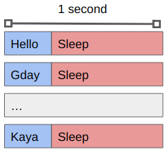
You’ll see that we get the same output as before (maybe in a different order) but that it occurs in batches of 8, with an approximately 1 second pause between them. What is happening now is that the waiting time is happening in parallel rather than in serial. If we replaced the sleep 1 command with some actual work that needs to be done then we’d be making use of multiple cores in no time!

By using a controller/worker approach, along with xargs, we can create a single job file that will spawn multiple tasks (up to some maximum) that will run concurrently. Moreover, if we have more tasks to complete than CPU cores available, xargs will wait for a task to complete before starting another.

Not everything can be parallelized

Some tasks are inherently serial and can’t be sped up by applying extra workers.

Two washing machines can’t wash a single load of clothes in 1/2 the time. This is because the wash/rinse/spin tasks are sequential and rely on each other.

Using multiple cores the hard(er) way

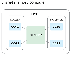
We have explored some ways of doing implicit multiprocessing by taking advantage of existing tools or libraries. We are now going to look at some of the explicit ways in which we can make use of multiple CPU cores at the same time. Any time we have a program that is working across multiple cores, we will in fact be working with a collection of processes (typically 1 per core), which are communicating with each other in order to complete the task at hand. Working with multiple cores or processes thus requires that we understand how to share information between processes, and thus we will discuss the two main paradigms - shared memory, and distributed memory.

Parallel processing with shared memory

In this paradigm we create a parent program which spawns multiple child processes, each of which have access to some common shared memory. This shared memory can be used for both reading or writing. In the second figure of the previous section, we could have a parent process spawning three children for a total of three active processes, using the following plan:

1. The parent process would create a shared memory location and read the input data into it, and then create an empty shared memory location for writing the output data.
2. The parent process would then spawn three children and pass them a reference to the shared memory locations, as well as information about which parts of the processing they will be responsible for (e.g. start/end memory address).
3. All three of the processes would then perform the same operation f(x) on different parts of the input array, and write to different parts of the output array.
4. When the parent process has completed it’s work it will wait for the children to complete theirs, and then write the output data to a file.

Each of the parent and child processes would run on a separate CPU core, and have their own memory allocation in addition to the shared memory.

The beauty of the above example is that the individual processes do not need to communicate or synchronize with each other in order to complete their work. Most importantly, they are never trying to read or write from the same memory address as each other. The only constraint is that all of the processes need to be able to directly reach the memory (RAM) in question, and this typically means that they all have to be running on the same node of an HPC. The scaling of your task is thus limited by the number of cores (and memory) available on a single node of the HPC facility.

Suppose that the function to be performed was to compute a running average of the input data over some window. In this case each of the processes would need to read data from overlapping regions of the input array (at the start/end of their allocation). Since the input data is not changing, having multiple concurrent reads is not an issue so each process can continue to act in isolation.

Suppose that the function we are performing is to build a histogram of the input data. The output data are then a set of bins initiated to zero, and the “function” is to read the bin, increment the value by one, and then write the result back to the output. Each of the processes can still read the input data without interfering with each other but now need to ensure that updating the output array doesn’t cause conflicts. For example, if two processes try to increment the same bin at the same time, then the’ll both read the same value (e.g. 0), increment it (to 1), and then write the result. One of these processes will write first and the other will write second, but the second one will overwrite the first. What we need in this case is a way to indicate that the read/increment/write part of the code can only be done by one process at a time. In this case we can use what is called a lock on the memory location. A process would lock a memory address, do the required read/increment/write, and then unlock the memory address. The library which provides the shared memory will track of all the locks, and if a process asks to use some memory space which is locked the process will be forced to wait until the lock is released before doing so. To avoid creating/releasing locks thousands of times, it would instead be useful to have each of the processes create their own version of the output data to work on locally, and then do the update once per bin when they are finished.

The OpenMP library is the most widely used for providing shared memory access to C and Fortran programs. Other languages (such as python) which provide shared memory libraries are either built on OpenMP or at least use the same programming paradigm and will therefore use similar terminology, and have similar limitations to OpenMP.

sky_sim_sharemem.py

#! /usr/bin/env python
# Demonstrate that we can simulate a catalogue of stars on the sky

import math
import numpy as np
import multiprocessing
from multiprocessing.shared_memory import SharedMemory
import uuid  # To generate unique strings
import sys

NSRC = 1_000_000
mem_id = None


# This function is run to initialize each of the new workers
# We need to pass the name of the shared memory so they can connect to it
def init(mem):
    global mem_id
    mem_id = mem
    return


def get_radec():
    # from wikipedia
    ra = 14.215420962967535
    dec = 41.26916666666666
    return ra,dec


def make_stars(args):
    # unpack args    
    ra, dec, shape, nsrc, job_id = args    
    # Find the shared memory and create a numpy array interface
    shmem = SharedMemory(name=f'radec_{mem_id}', create=False)
    radec = np.ndarray(shape, buffer=shmem.buf, dtype=np.float64)

    # make nsrc stars within 1 degree of ra/dec
    ras = np.random.uniform(ra-1, ra+1, size=nsrc)
    decs = np.random.uniform(dec-1, dec+1, size=nsrc)

    start = job_id * nsrc
    end = start + nsrc
    radec[0, start:end] = ras
    radec[1, start:end] = decs
    return


def make_stars_sharemem(ra, dec, nsrc=NSRC, cores=None):

    # By default use all available cores
    if cores is None:
        cores = multiprocessing.cpu_count()

    # 20 jobs each doing 1/20th of the sources
    # args are (ra, dec, shape, nsrc, job_id)
    args = [(ra, dec, (2, nsrc), nsrc//20, i) for i in range(20)]

    exit = False

    try:  # try/finally so that we always clean up the shared memory before exiting this function
        # set up the shared memory
        global mem_id
        mem_id = str(uuid.uuid4())

        # Determine the size of the memory required (in bytes)
        nbytes = 2 * nsrc * np.float64(1).nbytes

        # make the shared memory, with a unique name
        radec = SharedMemory(name=f'radec_{mem_id}', create=True, size=nbytes)

        # creating a new process will start a new python interpreter
        # on linux the new process is created using fork, which copies the memory
        # However on win/mac the new process is created using spawn, which does
        # not copy the memory. We therefore have to initialize the new process
        # and tell it what the value of mem_id is.
        method = 'spawn'
        if sys.platform.startswith('linux'):
            method = 'fork'
        
        # start a new process for each task, hopefully to reduce residual
        # memory use
        ctx = multiprocessing.get_context(method)
        pool = ctx.Pool(processes=cores, maxtasksperchild=1,
                        initializer=init, initargs=(mem_id,)
                        # ^-pass mem_id to the function 'init' when > creating a new process
                        )

        try:  # This try/except is to ensure that the pool is closed
            pool.map_async(make_stars, args, chunksize=1).get (timeout=10_000)
        except KeyboardInterrupt:
            print("Caught kbd interrupt")
            pool.close()
            exit = True # Note that something went wrong
        else:
            pool.close()
            pool.join()
            # make sure to .copy() or the data will disappear when you unlink the shared memory
            local_radec = np.ndarray((2, nsrc), buffer=radec.buf,
                                     dtype=np.float64).copy()
    finally: # Do all the cleanup
        radec.close()
        radec.unlink()
        if exit: # Quit if something went wrong
            sys.exit(1)
    return local_radec


if __name__ == "__main__":
    ra, dec = get_radec()
    pos = make_stars_sharemem(ra, dec, NSRC, 2)
    # now write these to a csv file for use by my other program
    with open('catalog.csv', 'w') as f:
        print("id,ra,dec", file=f)
        np.savetxt(f, np.column_stack((np.arange(NSRC), pos[0, :].T, > pos[1, :].T)),fmt='%07d, %12f, %12f')

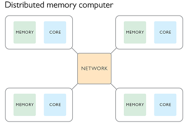
Parallel processing with distributed memory

In this paradigm we create a number of processes all at once and pass to them some meta-data such as the total number of processes, and their process number. Typically the process numbered zero will be considered the parent process and the others as children. In this paradigm each process has it’s own memory and there is no shared memory space. If we wanted to repeat the simple computing example used previously we would use the following plan:

1. All processes use their process number to figure out which part of the input data they will be working on.
2. Each process reads only the part of the input data that they require.
3. Each process computes f(x) on the input data and stores the output locally.
4. Each child process sends their output data to the parent process.
5. The parent process creates a new memory allocation large enough to store all the output data, and copies it’s own output into this memory.
6. The parent process then receives the output data from each child process and copies it to the output data array.
7. The parent process writes the output to a file.
8. All processes are now complete and terminate.

Each of the processes would run on a different CPU core and have their own memory space. This makes it possible for different processes to be run on different nodes of an HPC facility, with the message passing being done via the network.

It is still possible to have each process running on the same node. A message passing interface (MPI) has been developed and implemented in many open source libraries. As the name suggests the focus is not on sharing memory, but in passing information between processes. These processes can be on the same node or different nodes of an HPC.

The key to understanding how an MPI based code works is that all the processes are started simultaneously and then connect to a communication hub (usually called COMM_WORLD), they then execute the code. During code execution a processes can send/receive messages from any/all of the other nodes. A special type of message that is often used is called a barrier, which causes each process to block (wait) until all process are at the same point in the code. This is often required because, despite starting at the same time, the different processes can quickly get out of sync, especially if they need to perform I/O, communicate over a network, or simply have different data that they are working on.

Unlike with multiprocessing, the number of processes being used is determined outside of our code so we always have to ask questions like “how many processes are there total?” and “what is my process number?”. The process number is referred to as it’s rank and the only rank that is guaranteed to exist is 0, so this is often used as the special/parent rank.

sky_sim_mpi.py

#! /usr/bin/env python
# Demonstrate that we can simulate a catalogue of stars on the sky

# Determine Andromeda location in ra/dec degrees
import math
import numpy as np
from mpi4py import MPI
import glob

NSRC = 1_000_000

comm = MPI.COMM_WORLD
# rank of current process
rank = comm.Get_rank()
# total number of processes that are running
size = comm.Get_size()


def get_radec():
    # from wikipedia
    ra = 14.215420962967535
    dec = 41.26916666666666
    return ra,dec


def make_stars(ra, dec, nsrc, outfile):
    # make nsrc stars within 1 degree of ra/dec
    ras = np.random.uniform(ra-1, ra+1, size=nsrc)
    decs = np.random.uniform(dec-1, dec+1, size=nsrc)
    
    # return our results
    with open('{0}_part{1:03d}'.format(outfile, rank), 'w') as f:
        if rank == 0:
            print("id,ra,dec", file=f)
        np.savetxt(f, np.column_stack((np.arange(nsrc), ras, decs)),fmt='%07d, %12f, %12f')
    return


if __name__ == "__main__":

    ra,dec = get_radec()
    outfile = "catalog_mpi.csv"
    group_size = NSRC // size
    make_stars(ra, dec, group_size, outfile)

    # synchronize before moving on
    comm.Barrier()

    # Select one process to collate all the files
    if rank == 0:
        files = sorted(glob.glob("{0}_part*".format(outfile)))
        with open(outfile,'w') as wfile:
            for rfile in files:
                for l in open(rfile).readlines():
                    print(l.strip(),file=wfile)
                # os.remove(rfile)

This is run by calling python in a different way:

mpirun -n 4 python3 sky_sim_mpi.py

Our example above looks a lot simpler than the shared memory example, but this is because we have avoided passing any information between the different workers. We have used the rank of each worker to dictate what work it is doing. This is an ideal example. In general the coordinator and worker processes do need to communicate with each other, and this communication is done using the message passing interface (MPI). This interface is extremely inefficient at passing long messages, to the point where you can spend more time passing messages than doing work. The key to designing a good program with MPI is to keep the amount of message passing to a minimum.

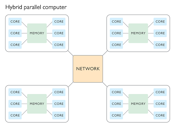
Hybrid parallel processing

It is possible to access the combined CPU and RAM of multiple nodes all at once by making use of a hybrid processing scheme. In such a scheme a program will use MPI to dispatch a bunch of primary processes, one per node, which in turn control multiple worker processes within each node which share memory using OpenMP.

Using many-many-many more cores (HPC)

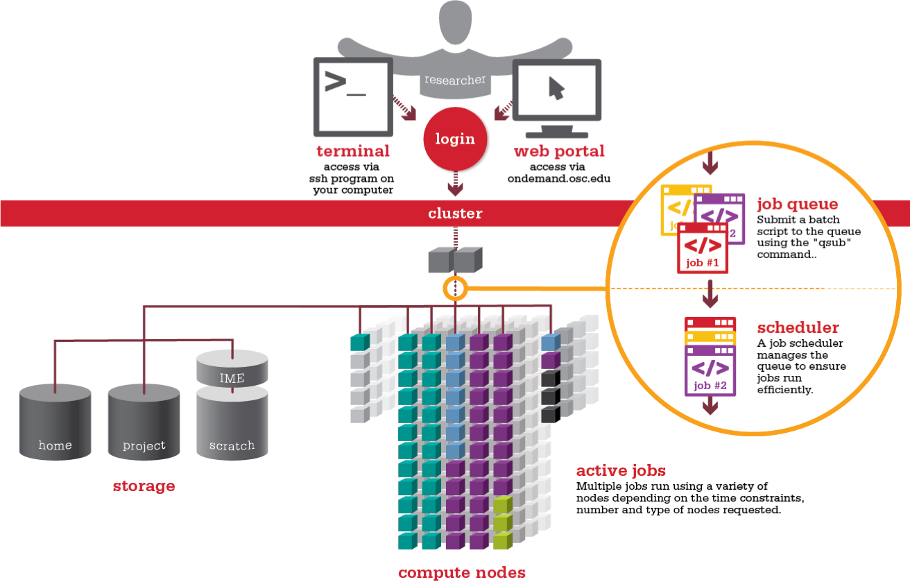
Most HPC systems have a layout something like the following:

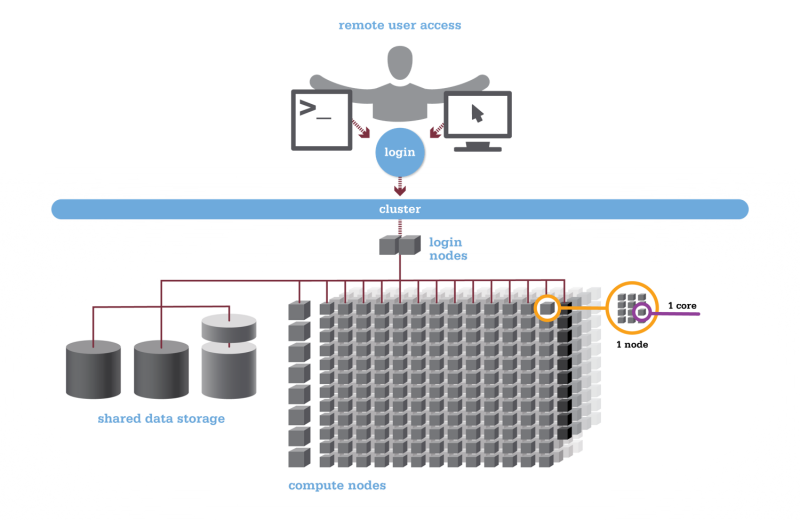
Different nodes

Typically you will log into one of a small number of login nodes via ssh. These nodes are not for doing any processing or work on, but are for you to write scripts, submit jobs, view the progress/status of your submitted jobs, and view the results of your work. These log-in nodes usually have similar hardware spec to a desktop machine (CPU/RAM wise) but will have have access to various shared file systems.

There are then compute nodes which are where all the work is to be done. These nodes typically have a large cpu or gpu count, a large amount of RAM, and possibly some super fast attached storage, in addition to being attached to the shared file systems. As noted before, the focus is on providing a large number of fast-ish cores, which means that the invidivual cores of an HPC will be slower than your desktop, but there will be orders of magnitude more cores available across the entire system. For example: Pawsey’s Setonnix system has 2.45GHz cores, but there are 64 per node, and 1600 nodes (102,000 cores) in total.

Making use of HPC

Aside from the hardware differences, the main difference is that your computer is just for your use. When you step away from your computer it will become idle waiting for you to return. Even when you are using your computer to browse the web or write emails, most of the hardware is not being used to it’s full capacity. Full screen, high intensity gaming can really give your computer a work out, pushing the compute, RAM, and maybe disk use to the maximum, but you personally cannot (and should not) sustain this activity 24/7. You might allow your computer to sleep or turn of when not in use to save some power. Suffice to say, that your computer has a lot of capacity to do work, but mostly it just renders web pages. This idle nature does not align with HPC’s goal of “always available, always working” so they are not operated this way. Any time an HPC resource is not being used is time / energy / money that is being wasted, and all HPC facilities will work to reduce this waste by maximizing use.

A shared use system is implemented such that many people can use the HPC resources at the same time. Not only can multiple people log into the system, but they each must plan the work that they will do and the resources that are required. One does this by submitting a computing job to a scheduler which will run your job once resources are available. The scheduling system figures out the most efficient way to complete all the work by minimizing the amount of resources (CPUs, RAM, GPUs, etc) that are unused.

The work scheduler is responsible for taking all of the work requests from all users, analyzing the resource requirements, scheduling where and when the jobs should be run, and then running those jobs. Commonly used schedulers are SLURM and PBS.

Migrating your workflow to an HPC can be a tricky task the first time you do it because the queue system adds an extra level of complexity to your work. For example, the scripts that you run for each trask in your workflow now need to have a bunch of extra information encoded in them so that the scheduler can run the script on your behalf. Additionally, you’ll need to tell the scheduler what resources you need: number of nodes, number of cores and RAM per node, and how long the job will run for.

If you are working entirely within a single compute node, then you can either use a single program with shared memory based parallelism, or make use of the controller/worker paradigm that we implemented with xargs. If you are wanting to work across multiple compute nodes at once, you’ll have to use MPI to communicate between nodes.

Depending on the HPC that you are considering to use there are some relevant ADACS training available at the following places:

• Pawsey + OzStar (SLURM based) ADACS training
• NCI (PBS based) ADACS training

Key Points

• Scaling resources can be more efficient than optimizing code.

• Effective use of multiple cores can significantly speed up research tasks.

• High-performance computing clusters offer powerful resources for research for a modest investment of time.

• Identifying and solving research bottlenecks can improve overall productivity.