Optimization
Overview
Teaching: 15 min
Exercises: 15 minQuestions
How can I optimize my code?
What am I even optimizing for?
Objectives
Review the different resources we can optimize for
Understand the optimization loop
Make our example code run at least a little faster
Scope your optimization work
When we are engaged in optimization there are a few things we should do first:
- Understand what the problem is
- Measure the current state of things (benchmark + first profile)
- Have a target in mind for what is “good enough”
When thinking about the problem, remember that your code doesn’t run in isolation. It runs as part of a larger workflow, that includes other pieces of code as well as non-automated things like researcher thinking time. Consider your entire workflow, and how much time is spent on waiting for code to run vs you analyzing results. If you have other useful work that can be done while your code runs, then do that, it’ll be time well spent.
Amdahl’s Law:
- System speed-up limited by the slowest component.
Paul’s rule of thumb:
- You are the slowest component.
Therefore:
- Focus on reducing your active interaction time,
- then on your total wait time,
- then on cpu time.
In parallel computing we’ll explore ways of making your work complete sooner, without making it run faster! Another way of making your code run faster can be to just buy a faster computer, though this isn’t always an option for everyone).
A reason to confirm that we need to optimize our code is that we want to avoid premature optimization:

Good coding practices can lead to more performant code from the outset. This is not wasted time.
Remember also that you cannot can’t optimize to zero. There will always be a minimum amount of time that your work will take to do, and you will only ever approach this minimum asymptotically. At first you’ll get 2-3 or even 10x speed increases for moderate effort, but as you keep going, you’ll end up spending a day writing unreadable code just for that 0.1% gain. Don’t be a speed addict, know when to quit!
Leveraging the work of others
There are a lot of python packages that are designed, directly or indirectly, to provide optimized python code. For example:
- NumPy
- The fundamental package for scientific computing with Python
- SciPy
- Fundamental algorithms for scientific computing in Python
- extends upon Numpy to provide additional data structures and algorithms
- Numba
- an open source JIT compiler that translates a subset of Python and NumPy code into fast machine code.
- Dask
- library for parallel computing in Python, with a focus on workflows and big data processing
- Taichi
- a domain-specific language embedded in Python that helps you easily write portable, high-performance parallel programs
- Cython
- an optimising static compiler for both the Python programming language and the extended Cython programming language
- write python code, convert it to c, compile, and run
- PyPy
- A fast, compliant alternative implementation of Python
- Not python modules will work in pypy, but many of the main one will
- pandas
- a fast, powerful, flexible and easy to use open source data analysis and manipulation tool, built on top of the Python programming language.
These packages can provide significant performance increases, often by implementing parallel processing under the hood, without you having to write or manage any of the parallel computing components.
The Optimization Loop
Using scalene we’ll re-run our initial profiling to ensure the results are consistent with the profiling we did in the previous lesson.
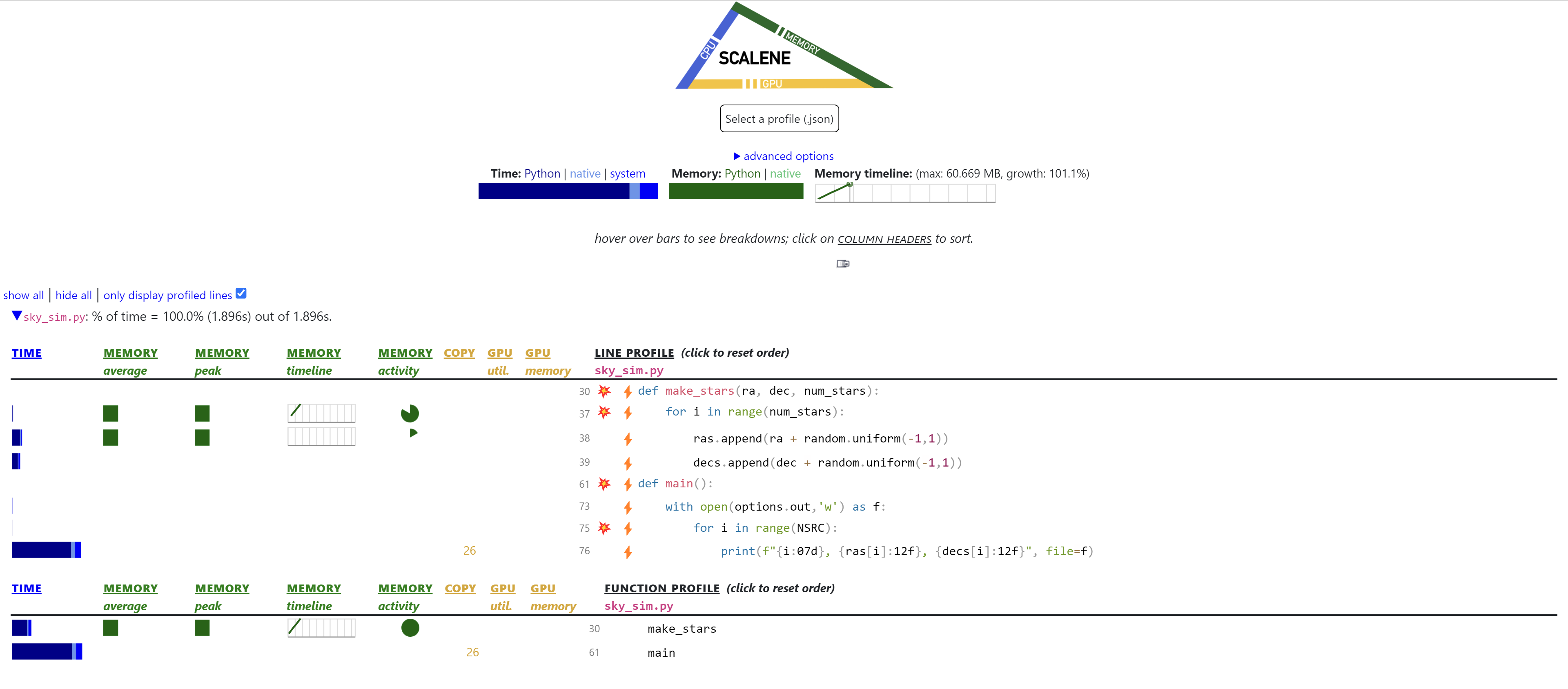
We should see the I/O is still the main bottleneck and as per Amdahl’s law we should fix that first.
One idea we can try first is to speed up the I/O (system) time by utlising the NumPy python module we are already using in several places.
NumPy has a way to quickly store data arrays into a file using the savetxt function.
For our exercise, we’ll create a new file in our mymodule directory and call it sky_sim_opt.py and copy the contents of your sky_sim.py into sky_sim_opt.py.
Using NumPy we can change the main function which runs all the functions to create our sources and then saves the csv file. To do this we’ll turn the ras and decs variables into
# Make sure to include an import to numpy as np at the top of your file.
import numpy as np

...

def main():
    parser = skysim_parser()
    options = parser.parse_args()
    # if ra/dec are not supplied the use a default value
    if None in [options.ra, options.dec]:
        ra, dec = get_radec()
    else:
        ra = options.ra
        dec = options.dec

    ras, decs = make_stars(ra,dec, NSRC)

    # Turn our list of floats into NumPy arrays
    ras = np.array(ras)
    decs = np.array(decs)
    # We stack the arrays together, and use savetxt with a comma delimiter
    np.savetxt(options.out, np.stack((ras, decs), axis = -1), delimiter=",")
    print(f"Wrote {options.out}")
Let’s rerun scalene without sky_sim_opt.py
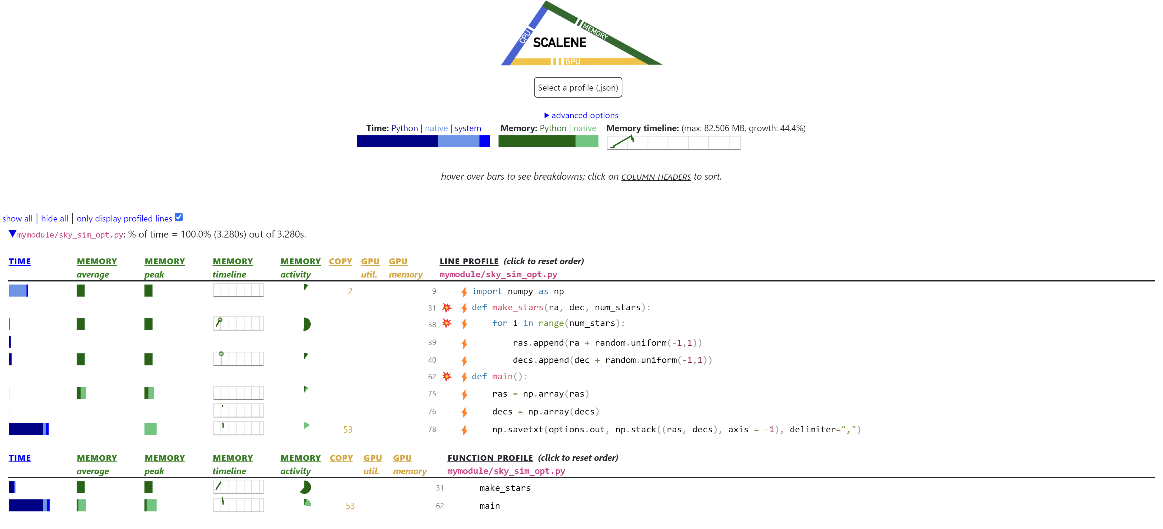
That is an unfortunate result, however we have increased the time spent in native which is a good thing. At the moment we are converting our list of floats into NumPy arrays, this has a cost of copying the lists from Python memory to the memory used for the native array in NumPy. The copying of arrays from Python to NumPy generally means it’s recommended that you start with NumPy arrays and then do operations on the arrays themselves using NumPy vectorized functions (we will cover vectorization more in parallel computing).
To initialize our arrays, most would suggest we initialize with an array containing only zeros using np.zeros, however because we are filling the array with values later, we can use a slightly faster operation np.empty. To show the difference between np.zeros and np.empty we can use the ipython %timeit magic. If you installed Python through Anaconda, ipython should already be installed, otherwise run pip install ipython. Inside your bash terminal run ipython, and run the following commands:
import numpy as np
%timeit np.zeros(1000000)
%timeit np.empty(1000000)
Python 3.8.16 | packaged by conda-forge | (default, Feb  1 2023, 16:01:55)
Type 'copyright', 'credits' or 'license' for more information
IPython 8.11.0 -- An enhanced Interactive Python. Type '?' for help.

In [1]: import numpy as np

In [2]: %timeit np.zeros(1000000)
317 µs ± 596 ns per loop (mean ± std. dev. of 7 runs, 1,000 loops each)

In [3]: %timeit np.empty(1000000)
278 ns ± 0.92 ns per loop (mean ± std. dev. of 7 runs, 1,000,000 loops each)
From the result of %timeit, we can see np.empty is measured in nanoseconds compared to microseconds for zeros, you’ll also notice np.empty completed 1000x more loops than np.zeros in the same amount of time, impressive! When comparing NumPy functions and functions that do similar things in general tools like %timeit are very useful. Tools like %timeit allows us to benchmark snippets of code to ensure our ideas of optimization do make sense (because having ideas is good, but testing them is even better).
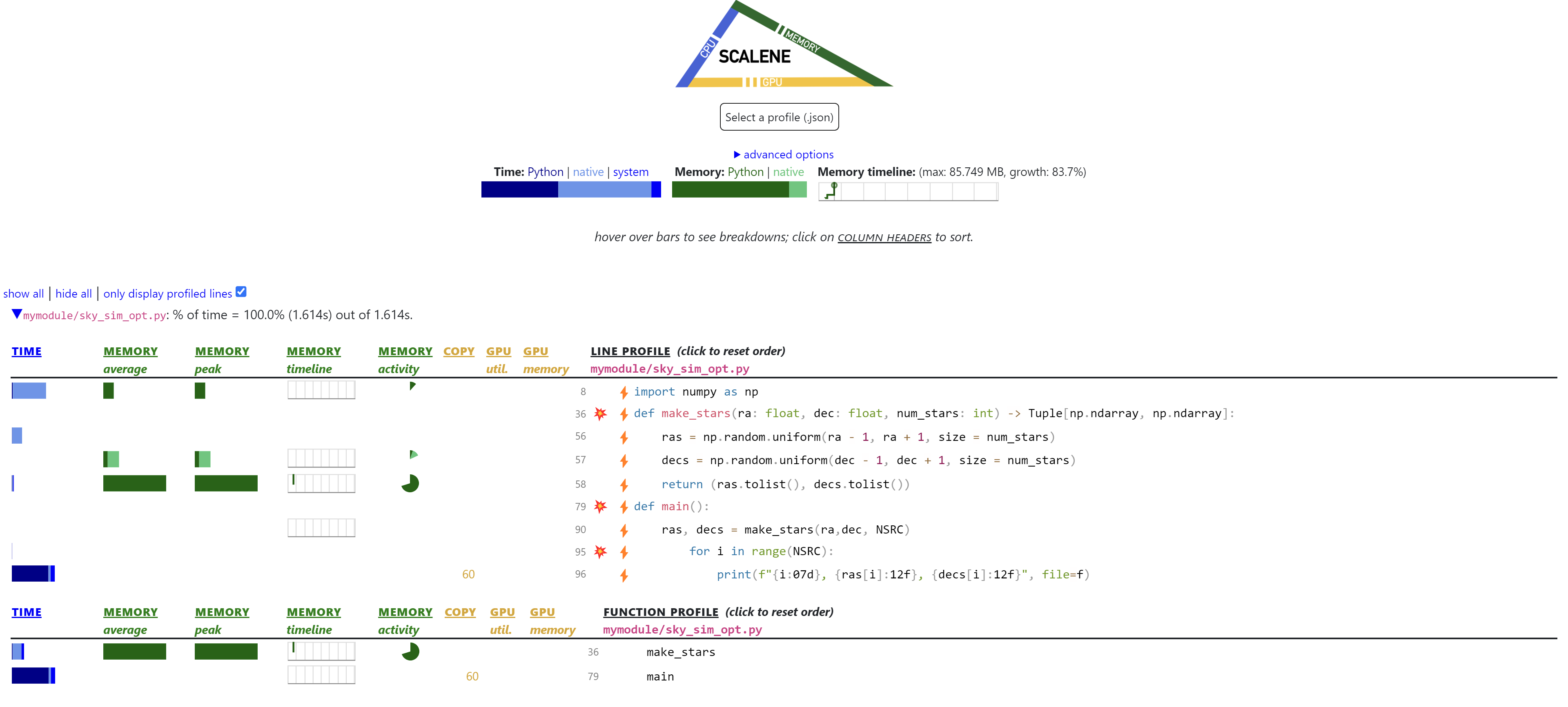
Although, as we look further into the NumPy documentation for more ideas we find the np.random.uniform function. This allows us to create a NumPy array of random values between a low and a high value of a certain size if we so wish. Using np.random.uniform we eliminate the comparatively slower Python for loop, and have make_stars run much faster.
Employing np.random.uniform change alongside our NumPy savetxt we get the following sky_sim_opt:
"""
A script to simulate a population of stars around the Andromeda galaxy
"""

# convert to decimal degrees
import math
import argparse
import numpy as np
from typing import Tuple

NSRC = 1_000_000

def get_radec() -> Tuple[float, float]:
    """
    Determine Andromeda location in ra/dec degrees

    Returns
    -------
    tuple(ra: float, dec: float)
        The Andromeda RA/DEC coordinate
    """
    # from wikipedia
    RA = '00:42:44.3'
    DEC = '41:16:09'

    d, m, s = DEC.split(':')
    dec = int(d)+int(m)/60+float(s)/3600

    h, m, s = RA.split(':')
    ra = 15*(int(h)+int(m)/60+float(s)/3600)
    ra = ra/math.cos(dec*math.pi/180)

    return (ra, dec)


def make_stars(ra: float, dec: float, num_stars: int) -> Tuple[np.ndarray, np.ndarray]:
    """
    Generate num_stars around a given RA/DEC coordinate given as floats in degrees.

    Parameters
    ----------
    ra : float
        The Right Ascension of the coordinate in the sky
    dec : float
        The Declination of the coordinate in the sky
    num_stars : int
        The number of stars we wish to generate

    Returns
    -------
    ras : np.ndarray, decs: np.ndarray
        A tuple of numpy arrays containing the RA and DEC coordinates in two arrays of the same size
    """

    # Making these as a numpy function allowed us to remove the comparably slow for loop, and take advantage of vectorization that numpy offers.
    ras = np.random.uniform(ra - 1, ra + 1, size = num_stars)
    decs = np.random.uniform(dec - 1, dec + 1, size = num_stars)
    return (ras.tolist(), decs.tolist())


def skysim_parser():
    """
    Configure the argparse for skysim

    Returns
    -------
    parser : argparse.ArgumentParser
        The parser for skysim.
    """
    parser = argparse.ArgumentParser(prog='sky_sim', prefix_chars='-')
    parser.add_argument('--ra', dest = 'ra', type=float, default=None,
                        help="Central ra (degrees) for the simulation location")
    parser.add_argument('--dec', dest = 'dec', type=float, default=None,
                        help="Central dec (degrees) for the simulation location")
    parser.add_argument('--out', dest='out', type=str, default='catalog.csv',
                        help='destination for the output catalog')
    return parser

def main():
    parser = skysim_parser()
    options = parser.parse_args()
    # if ra/dec are not supplied the use a default value
    if None in [options.ra, options.dec]:
        ra, dec = get_radec()
    else:
        ra = options.ra
        dec = options.dec

    # We are now returning numpy arrays
    ras, decs = make_stars(ra,dec, NSRC)

    # now write these to a csv file for use by my other program
    with open(options.out,'w') as f:
        print("id,ra,dec", file=f)
        for i in range(NSRC):
            print(f"{i:07d}, {ras[i]:12f}, {decs[i]:12f}", file=f)
    print(f"Wrote {options.out}")

if __name__ == "__main__":
    main()
You’ll notice the original code for writing a CSV is back.
Upon further investigation after changing to np.random.uniform we found that np.savetxt was slower than the code we had written previously.
This is a quick lesson in Python is a high level language and while we assume that packages such as NumPy always have faster functions, this isn’t always true as we don’t know what’s happening under the hood. This is why we described optimization as a loop, you’ll try ideas, some will work, others won’t, this is a natural part of the process. Sometimes though, code can’t be made faster quickly as we found out in the case here, we tried to find a faster way to write a CSV, and there probably is one, but we have declared it’s fast enough for our use case.
It’s time for you to see if you can make
sky_sim_optfasterIn your own time, feel free to try and see if you can optimize
sky_sim_opt.pyfurther, and if you do, let us know on the etherpad!
Bonus Note
Sometimes when optimizing code, you can encounter situations where your optimized code only runs faster in larger workloads, often optimizations employed may require the packages to do additional setup due to parallelization happening underneath or perhaps some memory wrangling needed underneath. Whatever the reason it may be, when benchmarking, profiling and optimizing your code it’s important you test the code under small and large workloads. Generally most optimize for the larger workloads rather than the smaller workloads, usually the extra setup cost for small workloads is worth it in comparison to the time saved on large workloads.
Key Points
After a while you’ll remember some of these optimization things and do them by default (esp, NumPy things)
Without profiling you are just guessing at what the problems is
Know when to stop