Parallel Computing

Overview

Teaching: 15 min
Exercises: 15 min

Questions

• What is parallel computing?

• How can I do parallel computing?

Objectives

• Understand the different types of parallelism

• Experience the joy of parallelism with xargs

• Understand different memory models for parallel processing

Intro

For many people parallel computing brings to mind optimization. Whilst optimization can often lead you down the path of parallel computing, the two are not the same. Parallel computing is about making use of resources while optimization is about making better use of the resources.

Types of parallelism

One of the biggest advantages of using an HPC is that you will have access to a large number of processing cores. These cores are often not that much faster than what you have on a desktop machine (they may even have a lower clock speed). A desktop machine will probably have between 4-12 CPU cores, where as the individual nodes of an HPC facility will have 24-48 cores, and of course there can be hundreds or thousands of such nodes within the facility. The key to making best use of HPC resources is thus organizing your work to make the best use of these multiple cores, and this means that you need to understand how to work in parallel.

There are many different levels of parallelism that you can work with, which we’ll explore now.

Task based parallelism

In task based parallelism we are working at the highest level of abstraction. In this model we take our workflow and break it into discrete tasks and then ask which tasks are independent of each other. These independent tasks can then be run at the same time in parallel. You may see these tasks referred to as embarrassingly parallel tasks.

Depending on how the software is implemented there are two main ways to run tasks in parallel:

1. Run one task per compute node, with many nodes being use at once. This would typically mean running an array job.
2. Run one task per CPU within a single compute node, with just one node being used at a time. This would be facilitated with a single job script.

We can of course run hybrid models which combine the two above extremes. Suppose we have 1000 tasks that need to be done, and each task can be completed using a single CPU core in 6hours. Suppose we want to run this on OzSTAR, such that we have 107 compute nodes, each with 36 CPU cores (of which we can use 32). We could use (1) above, but it would required 1,000 nodes x 6 hours of resources (6,000 node hours), and only use 1/36th of the available cores available on each node. This is not a good use of resources. We can’t use (2) above because our nodes don’t have 1000 cores in any single node. Instead we could divide our 1,000 tasks into 1000/32 = ~ 32 jobs, and then within each job run one task per CPU (assuming it will fit within the memory constraints of the node). This could be achieved by having a job array of 32 jobs, and each job would orchestrate the running of tasks numbered (n-1)*32 to (n-1)*32 + n, and making sure that the last job in the array stops at the 1,000th task. This method will result in 32 nodes x 6 hours of resources, or ~32 better than the previous option. We refer to this type of organization as job packing.

Here is a visualization of what we are doing: 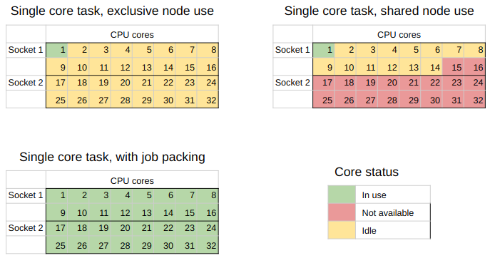In the top left we have the worst case scenario where a single user uses a node to run a task that uses just one core of the node. In the top right is a more realistic view of what happens when node resources can be shared. Multiple users can run jobs on the same node, but it’s not common that the requests people make are going to add up to 100% resource usage so there will be some wastage. In the bottom left is the goal that we are aiming for with job packing - complete use of all the CPU cores for the tasks we are running.

Occasionally, the limiting resource on a compute node is not the number of CPU cores but the amount of RAM available. If we can either limit or estimate the peak RAM usage of our tasks then we can adjust our job packing such that we use as much of the RAM as possible per node. For example, we might have 192GB of RAM available per node, but have a task that uses up to 10GB of RAM, and so we’d only be able to pack 19 copies of this task onto each of our compute nodes.

If we instead had 10,000,000 tasks that each took 20 second to run this would still have a total run time of approx 6,000 node hours, the same requirement as the previous example. However, SLURM takes some time to schedule a job, allocate resources, and then clean up when the job completes. This time is not that long (maybe 30 seconds), so if your job has a relatively short run time (few minutes) then this overhead becomes a significant overhead. In such cases we can pack our jobs such that we have 10,000 jobs running within a single job, but only 32 running at one time. This is a second form of job packing.

In each of the above implementations the parallelism is being handled by a combination of SLURM and our batch job scripts. We don’t need to have any knowledge of (or access to) the source code of the program that is actually doing the compute.

In a previous lesson we explored job arrays, so we won’t revisit them here, however we will dive a little deeper into job packing.

Job packing with xargs

The program xargs is standard on most Unix based systems and was created to “build and execute command lines from standard input”. At its most basic level, xargs will accept input from STDIN and convert this into commands which are then executed in the shell. xargs is able to manage the execution of these sub processes that it spawns and thus can be used to run multiple programs in parallel.

We will again simulate a hard task by doing something simple and then sleeping. In this case we have a script called greet.sh which is as follows:

greet.sh

#! /usr/bin/env bash

echo "$@ to you my friend!"
sleep 1

If we were to have a file which consisted of greetings (greetings.txt), one per line, we could use xargs to run our above script with the greeting as an argument:

xargs -a greetings.txt -L 1 -exec ./greet.sh

The -L 1 instructs xargs to pass one line at a time as arguments to our -exec command, and -a indicates the input data file. The above would eventually output the following:

Hello to you my friend!
Gday to you my friend!
Kaya to you my friend!
Kiaora to you my friend!
Aloha to you my friend!
Yassas to you my friend!
Konnichiwa to you my friend!
Bonjour to you my friend!
Hola to you my friend!
Ni Hao to you my friend!
Ciao to you my friend!
Guten Tag to you my friend!
Ola to you my friend!
Anyoung haseyo to you my friend!
Asalaam alaikum to you my friend!
Goddag to you my friend!
Shikamoo to you my friend!
Namaste to you my friend!
Merhaba to you my friend!
Shalom to you my friend!

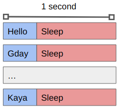
You’ll see that the sleep 1 command means that each greeting is followed by a pause, and that we only get one greeting at a time. The code is being executed on a single CPU core sequentially.

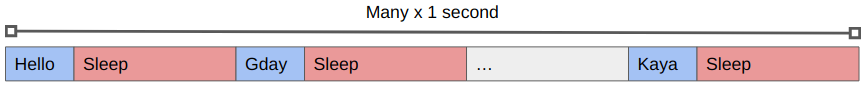
If we want to work with 8 tasks in parallel we can do so using the -P 8 argument to xargs:

xargs -a greetings.txt -L 1 -P 8 -exec ./greet.sh

You’ll see that we get the same output as before (maybe in a different order) but that it occurs in batches of 8, with an approximately 1 second pause between them. What is happening now is that the waiting time is happening in parallel rather than in serial. If we replaced the sleep 1 command with some actual work that needs to be done then we’d be making use of multiple cores in no time!

By using xargs we can create a single job file that will spawn multiple tasks (up to some maximum) that will run concurrently. Moreover, if we have more tasks to complete than CPU cores available, xargs will wait for a task to complete before starting another.

Vectorized operations

Vectorization is the process of rewriting a loop so that instead of doing one operation per loop over N loops, your processor will do the same operation on multiple data simultaneously per loop.

Modern CPUs provide support for this via what is called single instruction multiple data (SIMD) instructions. A CPU with a 512 register can hold 16x 32bit numbers at once (or 8x 64bits), and apply the same instruction to all of them within a single clock cycle.

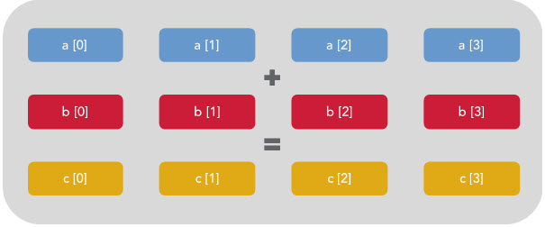
For example, if you wanted to add two vectors together, you could have a loop like this:

for (int i=0; i<16; i++)
  C[i] = A[i] + B[i];

Which would be executed on your CPU as like this if there is no vectorization happening:

You can see that only 1/4 of the register is being used. The rest is effectively wasted. However, if vectorization is enabled then the CPU will execute the same instruction on multiple data at once like this:

The above example is written in C rather than Python, because the C compiler is where this vectorization occurs. When compiled with the right flags, the C preprocessor will figure out which loops can be vectorized and rewrite them according to the data type and size / availability of the CPU register of the system that you are working on.

In a language like Python there is no compiler, just an interpreter, so how do we make use of vectorization? The answer is that we take our Python code, write it in C or Fortran, and then make a python wrapper function that will package our data up and send it to that code for processing. This is all rather fiddly work that most people don’t have time to do, so instead you should rely on libraries like numpy or scipy which are really python interfaces to fast, optimized, and often vectorized, C libraries.

Note that vectorization isn’t magic and it has some limits. The key thing to remember is that SIMD stands for SAME instruction multiple data. If your loop isn’t doing an identical operation every time then you can’t make use of vectorization. Things that break vectorization include: loop dependencies (accessing values after they have been changed in a previous iteration), flow control (if/break/continue statements within the loop), and calling functions within the loop.

In Python, the good rule of thumb is that vectorization is as simple as using numpy data structures and replacing your loops with to calls to numpy.

Vectorization with numpy

We’ll continue the above example with a python loop that computes C=A+B, where A and B are lists or arrays of integers. In this example we’ll show how we can complete the same operation using either Python list objects or numpy.array objects.

Add two python lists

Using ipython do the following and observe the output:

A_list=list(range(10_000))
B_list=list(range(10_000))

%timeit C_list = [ a+b for a,b in zip(A_list,B_list)]

Output

Depending on the speed of your computer you’ll get something like this:

529 µs ± 21.8 µs per loop (mean ± std. dev. of 7 runs, 1000 loops each)

Add two numpy arrays

Again using ipython, do the following and observe the output:

# assuming the same session as before
import numpy as np
A = np.array(A_list)
B = np.array(B_list)
%timeit C = A+B

Output

Depending on the speed of your computer you’ll get something like this:

1.18 µs ± 44.1 ns per loop (mean ± std. dev. of 7 runs, 1000000 loops each)

numpy contains more than just basic math functions. In fact many of the linear algebra operations that you would want to perform on arrays, vectors, or matrices (in the numpy.linalg module), call on powerful system level libraries such as OpenBLAS, MKL, and ATLAS. These libraries, in turn, are multi-threaded or multi-core enabled, so in many cases you’ll also be able to make use of multiple cores, without having to explicitly deal with the multiprocessing library, just by using numpy or scipy functions. Some particularly useful examples are the scipy.optimize and scipy.fft modules.

The main lesson here is that Python is slow but easy to code, and C is fast but hard(er) to code, but by using libraries such as numpy you can start to get the benefit of both worlds - easy to code, fast to use. So, wherever possible, use already built libraries and avoid re-implementing things yourself. Some potentially useful places to start are:

• numpy
• scipy
• astropy
• scikit-learn
• scikit-image

Share you favorite libraries

Share your favorite libraries with your group. Don’t restrict yourself to Python!

Domain or Data based parallelism

Consider an task that reads a data array, transforms it, and then writes it out again. The simplest implementation of such a task can be represented as follows, where f(x) represents the transform, and we iterate over all the data in order: 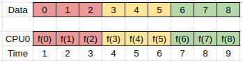In this example we have one compute unit (CPU0) doing all the work.

If multiple compute units are available (CPU0-2) then we can parallelize our work by having each compute unit perform the same set of instructions, but working on different parts of the data. We can then have these processes running in parallel as follows, and do the same work in 1/3 the time.

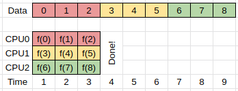
The above approach is often referred to as either domain or data based parallelism, because we are dividing our data into domains, and then working on each domain in parallel. Here we assume that the work that needs to be done to compute f(x_i) is independent of any previous results, or rather, that the order in which the results are computed is unimportant.

If our particular computing task falls into the above category, then we can replace our single processing design with a multiprocessing design in which all the processes that are doing the work have access to the same input/output memory locations. This form of parallelism requires that all the compute processes have access to the same memory which usually means that they all have to be on the same node of the HPC cluster that you are working on.

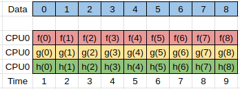
Another form of parallelism occurs when we have the same input data, but we want to process this data in different ways to give different outputs.

We could simply write completely different programs to perform the different calculations, but typically there is some preprocessing or setup work that needs to be done which is common between all the tasks. Here the separate tasks are represented by the functions f(x), g(x), and h(x), and can be run simultaneously.

In order to be able to implement the parallelism discussed here we need to understand how to share information between different processes. This is discussed in the next section.

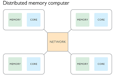
Memory models

We have explored some ways of doing implicit multiprocessing by taking advantage of existing tools or libraries. We are now going to look at some of the explicit ways in which we can make use of multiple CPU cores at the same time. Any time we have a program that is working across multiple cores, we will in fact be working with a collection of processes (typically 1 per core), which are communicating with each other in order to complete the task at hand. Working with multiple cores or processes thus requires that we understand how to share information between processes, and thus we will discuss the two main paradigms - shared memory, and distributed memory.

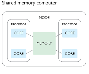
Parallel processing with shared memory

In this paradigm we create a parent program which spawns multiple child processes, each of which have access to some common shared memory. This shared memory can be used for both reading or writing. In the second figure of the previous section, we could have a parent process spawning three children for a total of three active processes, using the following plan:

1. The parent process would create a shared memory location and read the input data into it, and then create an empty shared memory location for writing the output data.
2. The parent process would then spawn three children and pass them a reference to the shared memory locations, as well as information about which parts of the processing they will be responsible for (e.g. start/end memory address).
3. All three of the processes would then perform the same operation f(x) on different parts of the input array, and write to different parts of the output array.
4. When the parent process has completed it’s work it will wait for the children to complete theirs, and then write the output data to a file.

Each of the parent and child processes would run on a separate CPU core, and have their own memory allocation in addition to the shared memory.

The beauty of the above example is that the individual processes do not need to communicate or synchronize with each other in order to complete their work. Most importantly, they are never trying to read or write from the same memory address as each other. The only constraint is that all of the processes need to be able to directly reach the memory (RAM) in question, and this typically means that they all have to be running on the same node of an HPC. The scaling of your task is thus limited by the number of cores (and memory) available on a single node of the HPC facility.

Suppose that the function to be performed was to compute a running average of the input data over some window. In this case each of the processes would need to read data from overlapping regions of the input array (at the start/end of their allocation). Since the input data is not changing, having multiple concurrent reads is not an issue so each process can continue to act in isolation.

Suppose that the function we are performing is to build a histogram of the input data. The output data are then a set of bins initiated to zero, and the “function” is to read the bin, increment the value by one, and then write the result back to the output. Each of the processes can still read the input data without interfering with each other but now need to ensure that updating the output array doesn’t cause conflicts. For example, if two processes try to increment the same bin at the same time, then the’ll both read the same value (e.g. 0), increment it (to 1), and then write the result. One of these processes will write first and the other will write second, but the second one will overwrite the first. What we need in this case is a way to indicate that the read/increment/write part of the code can only be done by one process at a time. In this case we can use what is called a lock on the memory location. A process would lock a memory address, do the required read/increment/write, and then unlock the memory address. The library which provides the shared memory will track of all the locks, and if a process asks to use some memory space which is locked the process will be forced to wait until the lock is released before doing so. To avoid creating/releasing locks thousands of times, it would instead be useful to have each of the processes create their own version of the output data to work on locally, and then do the update once per bin when they are finished.

The OpenMP library is the most widely used for providing shared memory access to C and Fortran programs. Other languages (such as python) which provide shared memory libraries are typically built on OpenMP and will therefore use similar terminology, and have similar limitations to OpenMP.

Be aware that SLURM needs to know how many CPU cores to allocate to your job. If you ask for --ntasks=1 then you’ll typically get just a single core. Use --ntasks=N or --cpu-per-task=N to have access to more cores.

An example inspired by the OzSTAR help and Wikipedia:

hello.c

#include <stdio.h>
#include <omp.h>

int main(void)
{
    #pragma omp parallel
    printf("Hello from process: %d\n", omp_get_thread_num());
    return 0;
}

We compile the above to produce our executable called hello:

gcc -fopenmp hello.c -o hello -ldl

We then run this with the following script:

openmp.sh

#! /usr/bin/env bash
#
#SBATCH --job-name=helloMP
#SBATCH --output=/fred/oz983/%u/OpenMP_Hello_%A_out.txt
#SBATCH --error=/fred/oz983/%u/OpenMP_Hello_%A_err.txt
#
#SBATCH --ntasks=1
#SBATCH --cpus-per-task=8
#SBATCH --time=00:01:00

# move to the directory where the script/data are
cd /fred/oz983/${USER}

export OMP_NUM_THREADS=$SLURM_CPUS_PER_TASK
/fred/oz983/KLuken_HPC_workshop/hello

In the our code hello.c we do not specify how many processes there will be. Instead we do this in the job script openmp.sh by setting 1 task, and 8 cpus-per-task. This will cause SLURM to allocate 8 cores to our job. From here the export statement will then tell OpenMP that we want to run this many threads, and we’ll end up with one thread (process) per core.

Run the openMP job

Run the job using sbatch openmp.sh and then when complete view the output file OpenMP_Hello_?_out.txt.

Results

Hello from process: 1
Hello from process: 7
Hello from process: 5
Hello from process: 0
Hello from process: 4
Hello from process: 6
Hello from process: 3
Hello from process: 2

Notice how the output doesn’t always occur in the order that we expect!

Parallel processing with distributed memory

In this paradigm we create a number of processes all at once and pass to them some meta-data such as the total number of processes, and their process number. Typically the process numbered zero will be considered the parent process and the others as children. In this paradigm each process has it’s own memory and there is no shared memory space. If we wanted to repeat the simple computing example used previously we would use the following plan:

1. All processes use their process number to figure out which part of the input data they will be working on.
2. Each process reads only the part of the input data that they require.
3. Each process computes f(x) on the input data and stores the output locally.
4. Each child process sends their output data to the parent process.
5. The parent process creates a new memory allocation large enough to store all the output data, and copies it’s own output into this memory.
6. The parent process then receives the output data from each child process and copies it to the output data array.
7. The parent process writes the output to a file.
8. All processes are now complete and terminate.

Each of the processes would run on a different CPU core and have their own memory space. This makes it possible for different processes to be run on different nodes of an HPC facility, with the message passing being done via the network.

It is still possible to have each process running on the same node. A message passing interface (MPI) has been developed and implemented in many open source libraries. As the name suggests the focus is not on sharing memory, but in passing information between processes. These processes can be on the same node or different nodes of an HPC.

In order for SLURM to initiate an MPI job it is essential for the user to indicate how many nodes and how many cores of each node will be used for the program. This is done via the --nodes and --ntasks options. Within a job script a user then starts the MPI part of their work using the srun command.

srun my_prog <args for my_prog>

Another example inspired by the OzSTAR help and Wikipedia. We compile the program into an executable called hello_mpi and then call it from the job script:

mpi.sh

#! /usr/bin/env bash
#
#SBATCH --job-name=helloMPI
#SBATCH --output=/fred/oz983/%u/MPI_Hello_%A_out.txt
#SBATCH --error=/fred/oz983/%u/MPI_Hello_%A_err.txt
#
#SBATCH --ntasks=8
#SBATCH --cpus-per-task=1
#SBATCH --time=00:01:00

# move to the directory where the script/data are
cd /fred/oz983/${USER}

srun /fred/oz983/KLuken_HPC_workshop/hello_mpi

Note here that we set ntasks to be 8, and use just one cpu per task. We no longer need to export anything, but we do need to use the srun command. The following output will be seen:

We have 8 processes.
Process 1 reporting for duty.
Process 2 reporting for duty.
Process 3 reporting for duty.
Process 4 reporting for duty.
Process 5 reporting for duty.
Process 6 reporting for duty.
Process 7 reporting for duty.

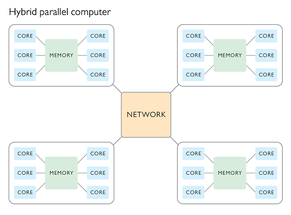
Hybrid parallel processing

It is possible to access the combined CPU and RAM of multiple nodes all at once by making use of a hybrid processing scheme. In such a scheme a program will use MPI to dispatch a bunch of primary processes, one per node, which in turn control multiple worker processes within each node which share memory using OpenMP.

Summary

There are many levels of parallelism that can be leveraged for faster throughput. The type of parallelism used will depend on the details of the job at hand or the amount of time that you are able and willing to invest. Starting with the easy parts first (eg job arrays and job packing with xargs) and then moving to shared memory or MPI jobs until you reach a desired level of performance is recommended.

Key Points

• Parallelism is not about optimization per se

• Understanding your workflow is key to planning your parallel processing

• Start with what is easy, make things harder only when necessary

• If using python leverage numpy data structures and functions