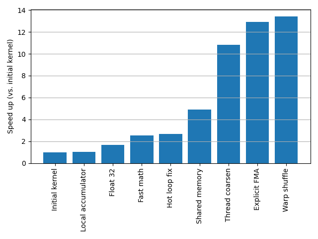
All in One View
Content from An introduction to parallelism
Last updated on 2026-07-15 | Edit this page
Estimated time: 40 minutes
Overview
Questions
- Why does adding more cores not always make a program faster?
- What distinguishes data parallelism from task parallelism, and why do GPUs rely on the former?
- Why does a parallel program sometimes give a different answer each time you run it?
Objectives
- Use Amdahl’s Law to estimate the maximum speedup achievable by parallelising a program.
- Identify code patterns that are safe to parallelise versus those that introduce data races.
- Write CPU-parallel code with Numba’s
@njitandprangeas a stepping stone to GPU kernels.
Why go parallel?
The short answer is speed.
You’ve probably heard of Moore’s Law, the observation that the number of transistors in a CPU doubles every two years. Up until the early 2000s, this law held true for the single-core CPUs of the time. Processor speeds increased from being measured in mere kHz, to MHz and finally to GHz. But physical limitations, and in particular power draw and heat, put a stop to those increases. CPU cores today have clock speeds measured in the same single digit GHz range as they did 25 years ago (with only marginal gains coming from instruction efficiencies).
Moore’s Law has continued unabated, but those extra transistors have spilled over into multicore CPUs and GPUs. Serial programs that execute one instruction at a time gain nothing from this shift. Increasing performance must come instead through parallelism: doing more work simultaneously, rather than doing each piece of work faster.
GPUs take this to an extreme. GPU parallelism trades latency for throughput: any single GPU core is considerably slower than a modern CPU core, but a GPU can run tens of thousands of tasks simultaneously. If your problem can be decomposed into many independent units of work, a GPU can process all of them in far less total time than a serial CPU could manage.
Amdahl’s Law
Amdahl’s Law formalises what is a very obvious observation. Consider an example where 80% of your computation is parallelisable. Then no matter how many threads you throw at a problem, that remaining 20% represents a hard floor. With only 4 cores, the actual speedup is closer to 2.86x — significantly less than the 4x you might naively expect.
More formally, the speed up, \(S\), is given by:
\[S = \frac{1}{(1 - p) + \frac{p}{N}}\]
where \(p\) is the fraction of the program that can be parallelised, and \(N\) is the number of parallel execution units (cores, threads, etc.).
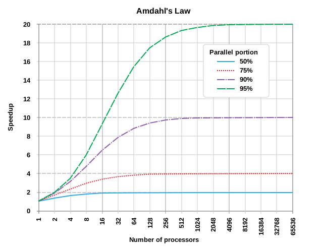
Credit: Daniels220 at English Wikipedia
The practical takeaway: parallelism delivers the most benefit when the parallelisable portion of your code is both large and dominates the runtime. If your bottleneck is I/O or your algorithm is principally serial in nature, throwing more cores at it will do little.
Challenge
Think about your own code: which parts are parallelisable and which are fundamentally serial? Can you provide an estimate of the kinds of speedup you could expect?
Task parallelism versus data parallelism
Parallel code comes in two principal forms.
Task parallelism
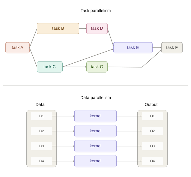
Task parallelism divides work into different types of jobs. Each task functions autonomously and relies on communication between tasks to coordinate.
Example: Consider building a bike: one person assembles frames, another builds tyres, and a third puts it all together. This series of specialised tasks is one form of task parallelism known as pipelining. Another is a worker pool: each person builds a complete bike from scratch, but (possibly) to a different customer specification.
Task parallelism requires careful coordination — semaphores, mutexes, locks, message passing, and other synchronisation primitives. This coordination is a common source of bugs.
Task parallelism is the principal model of threaded operations on the
CPU (e.g., Python’s threading or
multiprocessing modules, or C’s OpenMP tasks).
Data parallelism
Data parallelism applies the same computation to many independent pieces of data. Each thread performs identical work on variable inputs.
Example: Applying a filter to every pixel in an image. The filter is the same; the pixel data differs.
Data parallelism is implemented in hardware on the CPU as “single instruction, multiple data” (SIMD) — for example, AVX or SSE instructions that operate on vectors of data within a single CPU register. On the GPU it is implemented as “single instruction, multiple thread” (SIMT) — the same concept scaled to tens of thousands of threads.
This programming model is quite restrictive:
- The computation must be identical for each data element.
- Communication between threads is very limited; each thread should proceed independently.
- Threads ideally proceed in lockstep — branches that cause threads to diverge can be costly.
GPUs are built around data parallelism and derive much of their speed advantage from the restrictive model and the simplicity it affords to both the hardware and software implementations.
Throughout this workshop we focus exclusively on data parallelism. The GPU is a data parallel machine, and the kernels you will write are data parallel kernels.
An introduction to Numba
To experiment with data parallelism on the CPU before moving to the GPU, we are going to use Numba. Numba is a just-in-time (JIT) compiler that translates annotated Python code into fast, machine-level code.
JIT compilation means that the translation happens at runtime: the first time a decorated function is called, Numba compiles it based on the argument types. Subsequent calls reuse the compiled version, so the compilation overhead is paid only once. The same JIT mechanism is used later when we write GPU kernels — the kernel is compiled to CUDA code on first call and cached thereafter.
Numba will be fundamental to our later workflows for writing GPU kernels: we first write the kernel on the CPU, verify that it works when run in parallel in Numba, and finally shift the code onto the GPU.
The JIT compiler used in Numba (and later in CUDA) compiles code at
the function boundary. When the function is first called, the compiler
will first inspect the types of each of the function’s arguments
(e.g. int, float, or perhaps
np.array(dtype=complex)). Based on these input types, the
types of the whole function are then inferred and finally the
function is compiled to machine code. This compilation takes a little
time (a few hundred ms or so), but only needs to be done once. Next time
the function is called, and the types match, the cached function will be
used.
You might also sometimes see @njit code with type
annotations in the decorator. Whilst these have no effect on performance
they may be useful as documentation or in ensuring argument types match
expectations.
The @njit decorator
The simplest way to use Numba is the @njit decorator,
which compiles a function into optimised machine code:
PYTHON
from numba import njit
import numpy as np

@njit
def add(xs, ys, zs):
    for i in range(len(xs)):
        zs[i] = xs[i] + ys[i]

N = 1_000_000
xs = np.random.normal(size=N)
ys = np.random.normal(size=N)
zs = np.empty(N)

add(xs, ys, zs)
np.testing.assert_allclose(zs, xs + ys)
The function looks like ordinary Python, but after JIT compilation it runs at near-C speed. Numba supports a substantial (but limited) subset of Python: loops, conditionals, numpy array access, and many math functions. It does not support most Python object-oriented features or dynamic typing.
Note that we allocated the memory (xs, ys,
and zs) outside the function. Just as we will see
later with CUDA kernels, it is best to pre-allocate Numba arrays in
regular Python and pass them in as arguments, with one of those
arguments typically used to write the function output.
Parallel loops with prange
Numba’s prange (parallel range) is the easiest way to
write data parallel code. It tells Numba to distribute each of the loop
iterations across CPU threads:
PYTHON
from numba import njit, prange
import numpy as np

@njit(parallel=True)
def add(xs, ys, zs):
    for i in prange(len(xs)):
        # Things run in parallel inside the prange loop
        zs[i] = xs[i] + ys[i]

N = 1_000_000
xs = np.random.normal(size=N)
ys = np.random.normal(size=N)
zs = np.empty(N)

add(xs, ys, zs)
np.testing.assert_allclose(zs, xs + ys)
Two things changed here:
- We use
prangefor the loop instead of the regularrange. - We set
parallel=Truein the decorator which enables special functions—likeprange—to run in parallel. (But it does not make the whole function run in parallel.)
Each iteration of the loop is independent — thread i
reads from and writes to index i, and no other thread
touches that index. This is the hallmark of a good data parallel
problem: the work is decomposed into independent units that can proceed
in any order.
Keep in mind that while prange looks like
range, the iterations are not guaranteed to execute in
order nor are they guaranteed to execute all at once. Numba decides how
to distribute the work across available CPU threads.
Challenge
Write a prange-parallel function that computes the
element-wise square root of an array. Verify correctness against
numpy.sqrt.
PYTHON
import numpy as np
from numba import njit, prange

@njit(parallel=True)
def parallel_sqrt(xs, ys):
    # TODO: use prange to fill ys with the square root of each element of xs
    pass

xs = np.random.uniform(0, 10, size=1_000_000)
ys = np.empty_like(xs)
parallel_sqrt(xs, ys)
np.testing.assert_allclose(ys, np.sqrt(xs))The pitfalls of parallelism
Parallel code promises increased performance but it comes with some real costs too. For example:
- Not everything parallelises. Some parts of your algorithm may inherently depend on results from earlier steps. These inherently serial aspects of your code place strict limits on the effects of parallelisation (see Amdahl’s law).
- Parallel code is harder to reason about. Parallel code is usually more complex to write. It is also harder to understand: with multiple threads executing at once, the order of operations is no longer guaranteed.
- More complexity means more bugs. Parallelism introduces an entirely new class of errors — data races — that appear when threads compete for shared resources.
- Parallel code introduces its own costs. There is an overhead cost to managing and scheduling multiple threads; and there can arise resource bottlenecks for memory or I/O.
Something that we will stress repeatedly throughout this course is that you must carefully weigh these costs against any possible performance gains. Be selective in what is parallelised, and always consider performance improvements in terms of the lifecycle of the entire program (and that includes development time too!).
Data races
The most insidious class of bugs in parallel code is the data race. A data race occurs when two or more threads access the same memory location concurrently, and at least one of them is writing — with no synchronisation between them.
Consider this attempt at a parallel sum:
PYTHON
@njit(parallel=True)
def racy_sum(xs):
    # We initialise x_sum as a single element array to stop Numba from fixing our
    # race condition. If we used a scalar value, e.g. by initialising x_sum = 0;
    # then Numba will secretly fix our race condition.
    x_sum = np.zeros(1)
    for i in prange(len(xs)):
        # Parallel sum
        x_sum[0] += xs[i]
    return x_sum[0]

xs = np.ones(1_000_000)
print("Sum:", racy_sum(xs))
# Expected: 1000000.0
# Actual:   ? (likely wrong, and varies each run!)
The problem is that x_sum[0] += xs[i] is not a single
operation — it is three:
-
Read the current value of
x_sum[0]. -
Add
xs[i]to it. -
Write the result back to
x_sum[0].
With multiple threads executing these steps simultaneously, threads can read a stale value before another thread has written its update. The result is lost, and the final sum is incorrect — and nondeterministic, varying from run to run.
Race conditions occur in any situation where multiple threads access shared and mutable state of some kind.
Challenge
Run the racy_sum function several times. Does it always
return the same result? Does the result change if you increase the size
of the input array?
One approach to resolving this problem is to give each thread its own accumulator:
PYTHON
from numba import njit, prange, get_num_threads, get_thread_id

@njit(parallel=True)
def safe_sum(xs):
    # Each thread gets its own slot
    x_sums = np.zeros(get_num_threads())

    for i in prange(len(xs)):
        # Parallel sum, but each thread writes to its own slot
        x_sums[get_thread_id()] += xs[i]

    # Serial reduction of per-thread sums
    return x_sums.sum()

xs = np.ones(1_000_000)
print("Sum:", safe_sum(xs))  # 1000000.0 — correct and deterministic
Each thread writes only to its own index, so there is no contention. The final serial reduction is cheap because there is one entry per CPU thread (typically fewer than 64).
Performance overhead
Parallel code doesn’t come for free. In fact, sometimes throwing more threads at a problem can make things slower.
The types of overhead differ between CPU and GPU. When using CPU-backed threads, some of the costs include:
- Thread spawning: which involves creating a thread and allocating it some initial memory
- Context switching: when there are more threads than cores, the host OS will periodically suspend threads to “fairly” let each thread advance its work
- Communication overhead: all higher level communication methods are built on a toolbox of atomics, locks, semaphores and condition variables and these have a non-negligible overhead
On the GPU, the costs are different — owing mostly to the fact that the CPU (the “host”) and the GPU (the “device”) are physically distinct. Some of these costs include:
- Memory transfers: GPUs have their own memory that is separate from the host and it takes time to transfer back and forth
- Command latency: telling the GPU what to do and transferring kernels has some associated latency
- Synchronisation and communication: a GPU has its own synchronisation primitives and a limited ability to communicate, both of which have a cost
When designing GPU code you must ensure that the computational benefits dwarf the associated costs of memory transfers and ensure your algorithm uses synchronisation sparingly.
In addition, your algorithm may also be slowed down by resource contention. This occurs when different threads all attempt to access a single resource of some kind, perhaps a file on disk, a network resource, or even to access memory. Slow downs due to resource contention can sometimes be non-linear (known as performance cliffs).
Code complexity
Serial code is very easy to reason about: first this happens, then this, and finally that. Under the hood, the compiler may perform all sorts of optimisations (e.g. rearranging the order of instructions or pre-emptively executing a conditional branch) but it does this whilst guaranteeing that these are invisible within the thread.
Parallel code tends to be much more complex:
- Each thread is doing only part of the overall computation
- You can no longer guarantee the ordering of operations: threads may start, suspend, and stop at different times
- Compiler optimisations become visible between threads
- Significant programmer work is required to reason about and handle synchronisation
These complexities mean that bugs are more likely, and you must weigh this against the performance benefits you expect.
Always write your algorithm in a single threaded, serial form first, and use this to test your parallel code later for correctness.
Challenge
Consider the following simple Python loops. Which of these is safe to
parallelise with prange, and if not, why not.
PYTHON
# A
for i in range(len(xs) - 1):
    ys[i] = xs[i] ** 2 + xs[i + 1]**2

# B
for i in range(1, len(xs)-1):
    ys[i] = (xs[i-1] + xs[i+1]) / 2   # read from xs, write to ys

# C
for i in range(len(xs)):
    if xs[i] > threshold:
        indices.append(i)

# D
x_min = xs[0]
for i in range(len(xs)):
    if xs[i] < x_min:
        x_min = xs[i]

# E
for i in range(len(xs)):
    if xs[i] > 0:
ys[i] = math.sqrt(xs[i])- A is safe: threads read from the same values, but since these are not changed this is not a race condition.
- B is safe: reads and writes to different arrays.
- C is not safe: appending to an array mutates shared state.
- D is not safe: there is a race condition on the shared and mutable
x_minvalue. - E is safe: conditional is per-thread, no shared state.
Content from A GPU Deep Dive
Last updated on 2026-07-15 | Edit this page
Overview
Questions
- How is a GPU organised internally, and how does that differ from a CPU?
- Why does the GPU have multiple types of memory with very different speeds and sizes?
- How does a GPU avoid sitting idle while waiting for slow memory operations?
Objectives
- Describe the GPU hardware hierarchy: streaming multiprocessors, cores, warps, and thread blocks.
- Explain the GPU memory hierarchy and when to use registers, shared memory, or global memory.
- Describe how latency hiding uses massive concurrency to keep GPU cores busy.
A little history
Graphics Processing Units (GPUs) were originally built to offload 2D and 3D visualisation computation from the CPU onto a dedicated device. The nature of video processing workloads meant that GPUs were built to handle data parallel workloads from the start. As GPUs became increasingly sophisticated, especially with the advent of programmable shaders and floating point support, it became apparent that GPUs offered the potential to perform general purpose computation (GPGPU). As early as 2003 there were already papers demonstrating how GPU graphics primitives could be repurposed to perform linear algebra.
NVIDIA formalised this general purpose computing on its GPUs with its release of the CUDA library in 2006. Much later in 2016, AMD released ROCm which provided a similar GPGPU interface to its own hardware. There are also open source APIs including OpenCL and SYCL, Microsoft’s OneAPI which claims to bridge a range of accelerators, as well as AMD’s cross-platform compatibility layer known as HIP. Despite these offerings, there remains strong vendor lock-in, and NVIDIA and its proprietary CUDA API remains dominant.
Today, GPUs have diverged somewhat in their design depending on whether they are destined to function as a true graphics processing device or as more general purpose compute accelerator. Increasingly, AI workloads are driving design decisions that might not be useful for (or even harm!) some scientific workloads.
The GPU
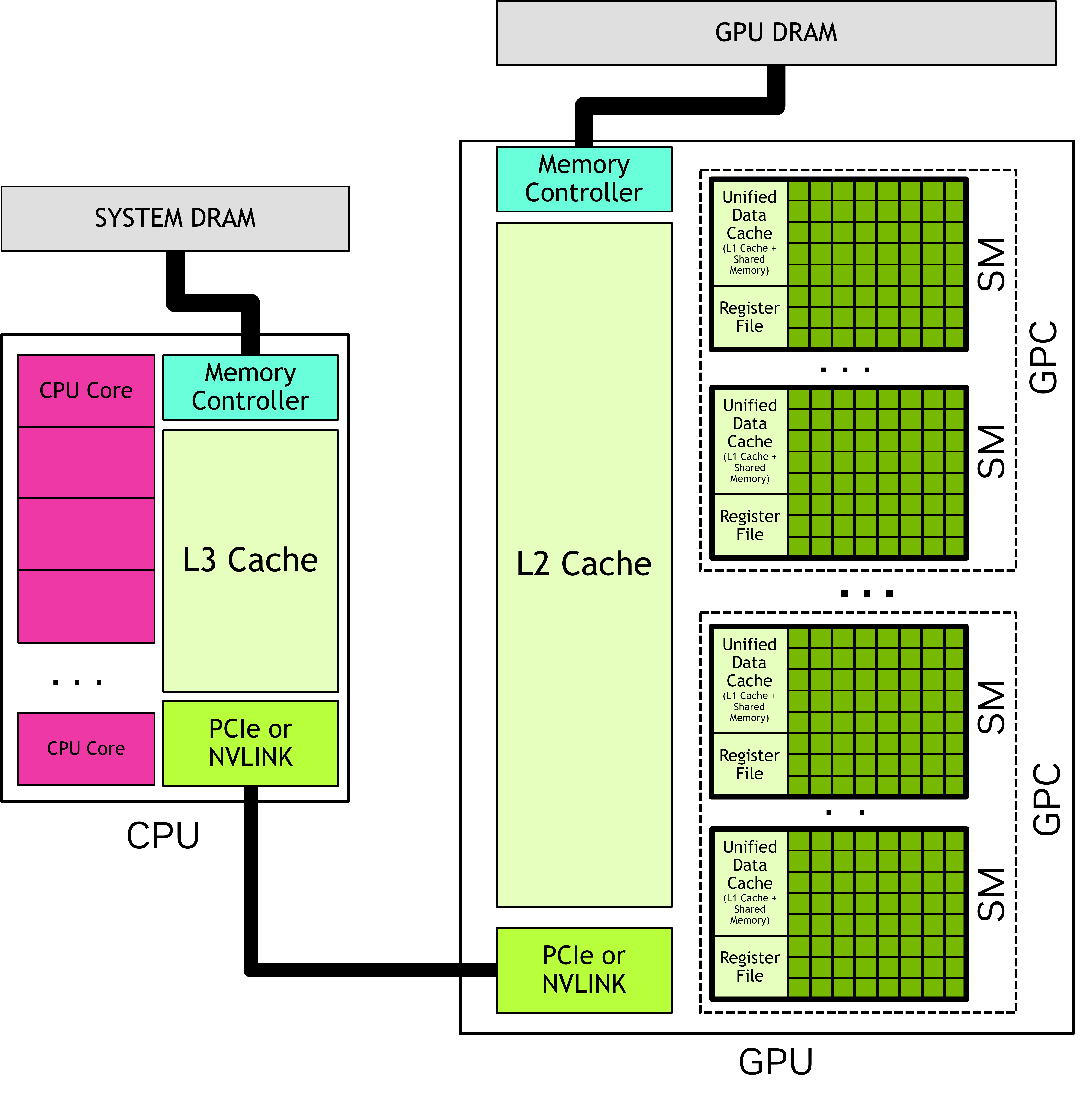
In most systems, the GPU is physically distinct from the CPU. It has its own computing cores, its own memory, its own floating point units, its own controllers, and a number of other units. The CPU and the GPU communicate with each other across some kind of serialisation link such as PCIe.
Oftentimes you will see the CPU referred to as the host, and the GPU referred to as the device. This language should stress the separation of these two domains.
In the simplest terms, a GPU is two things:
- Parallel compute, provided by numerous streaming multiprocessors (SM), each of which in turn hosts numerous cores (and other resources)
- Memory, at a range of tiers that includes DRAM (“global”), SRAM (“shared”), registers and numerous caches
Streaming multiprocessor
A streaming multiprocessor (SM) is a collection of cores that are grouped together and share some resources in common. Take for example the recent NVIDIA B200 GPU: this has 148 SM, and each SM has 128 cores.
GPU cores (sometimes called a ‘CUDA cores’, or ‘shader processors’) are like the cores on your CPU but differ in some important ways:
- They are individually slower. The B200, for example, has clock speeds of only 700 MHz. In highly parallelisable computations, thousands of slow cores tend to be faster than a handful of very fast cores.
- They are much simpler in design.
- They are physically smaller, mostly as a result of being slower and simpler.
- They don’t have their own register space. Registers are the small “scratch pad” of memory that is immediately accessible by a core. On a CPU, the register is attached to the core, with the downside that if a thread moves between cores it must also move the register memory. On a GPU, the register space is shared by the SM, which makes it easy to suspend and resume threads with little overhead.
- They always run in SIMD/SIMT mode. Threads are grouped together into batches of 32 (or 64 on AMD hardware) known as a warp and assigned to run in lockstep.
A SM has a number of resources shared amongst the cores. We’ve already seen that the register space is shared. In addition, it has a shared floating point unit (FPU) where, just like on the CPU, when floating point math needs to be performed, the work will be delegated to this shared unit. Unlike on CPUs, these FPUs also have specialised hardware for computing some more complex math functions, like exponents, logarithms and trigonometry. More modern GPUs also have tensor cores which are specialised for matrix operations.
You might ask, why have the streaming multiprocessor at all? Why have this intermediary entity in the hierarchy between the GPU and the cores themselves? The answer: physical locality. A GPU is a physical device and distance matters. By grouping the cores and assigning each a set of shared resources that reside nearby on the die, we can make their use cheaper and faster.
Understanding memory
The GPU has its own memory that is distinct from the host memory. In fact, the GPU can’t “see” host memory (and vice versa) and memory must be transferred back and forth between host and device depending on where it is needed.
The GPU has multiple layers of memory, each with different trade offs:
| Memory type | Operation | Visibility | Size | Speed |
|---|---|---|---|---|
| Global | Manual | All threads | Tens of GBs | Slow |
| Shared | Manual | Thread block | Hundreds of KBs | Fast |
| Registers | Manual | Thread | Hundreds of KBs | Fastest |
| L1 Cache | Automatic | SM | Hundreds of KBs | Fast |
| L2 Cache | Automatic | All threads | Tens of MBs | Moderate |
Global memory is where all input data must start and ultimately where the results of any computation must be written. When we transfer memory from host to device, or back again, we are using global memory. It is the largest store of memory on the GPU and is visible by all threads on the GPU. It is fully controlled by the host: the host allocates the memory and chooses when to destroy it. It thus outlives any kernels that run in the interim.
Shared memory is a much smaller pool of transient memory that can be utilised by a thread block, and which lives only as long as the thread block. Shared memory resides within the SM itself and is much faster than global memory. Shared memory is often used by thread blocks as a shared cache or as a means to communicate and coordinate work.
Registers are the collection of individual variables used by a single thread. For example, a register might be used by a loop counter, or to store an intermediate calculation, or to cache a value from global memory so that it can later be used. Registers exist only for the life of the thread and are visible only to itself. Unlike with CPUs, registers aren’t attached directly to processing cores, but are shared by the entire SM: this allows a warp to be paused and later continued on any of the SMs cores without worrying about transferring registers.
(Register spills occur when a thread uses so many registers that they can’t all fit in the SM. When this happens, the compiler (silently) lets some of the registers “spill” into global memory. These values are referred to as local memory: they’re accessible only by the thread even though they are physically stored in global memory. Needless to say, you will want to avoid register spills as they are terrible for performance.)
The remaining memory types are caches that are automatically populated and managed by the device. They may make commonly accessed parts of global memory faster, depending on the caching policy in effect.
Understanding the different types of GPU memory is crucial to GPU optimisation work. In general, we want to write code that minimises slow global memory operations as much as possible, swapping these for much faster shared or register memory operations.
(Image: Subramaniyam Pooni)
The grid
When launching a computation on the GPU, you must first configure its grid. A grid consists of:
- A configurable number of threads. Threads are the fundamental unit of parallelisation and are usually numbered in the millions.
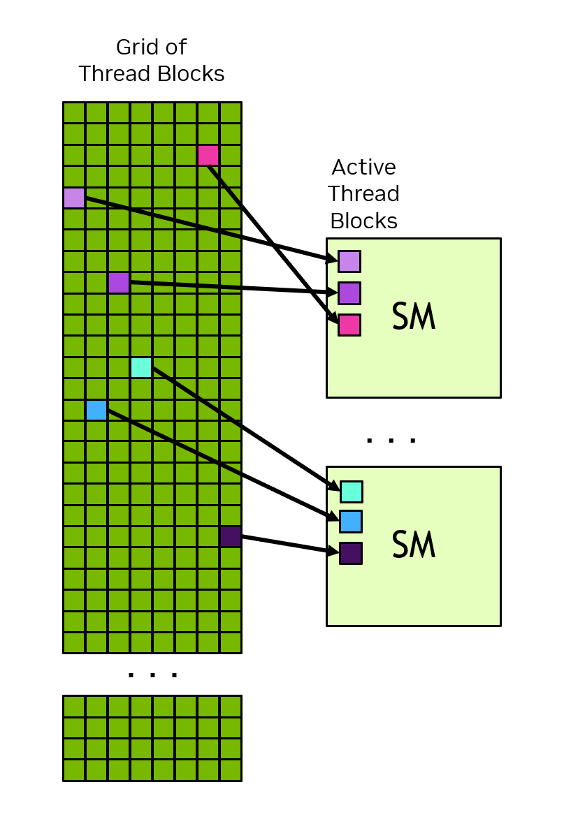
- Threads are grouped together into thread blocks, each thread block having a fixed number of threads.
- Finally, the collection of thread blocks forms the grid.
You might wonder, why do we have thread blocks? The reason: thread blocks are executed on a single SM, and this gives their threads special powers. In particular, this allows threads within a thread block to communicate and coordinate with each other quite efficiently, which is often essential for many types of problems.
This software hierarchy of grid > thread blocks > threads has a corollary in the hardware hierarchy of GPU > SMs > cores, but it’s important to keep in mind that they are separate concepts:
- You can have vastly many more thread blocks than SMs: thread blocks are enqueued to SMs when they have capacity, and each SM usually has a number of thread blocks enqueued at any one time.
- Similarly, the number of threads you can configure can be vastly larger than the physical cores. In fact, for reasons of performance (see: latency hiding) this is usually preferable.
- Thread blocks don’t need to be multiples of the warp size, e.g. multiples of 32. You can size your thread blocks arbitrarily, up to the hardware-imposed limit of your GPU. Although for performance reasons you probably shouldn’t!
Why thread blocks?
The GPU hardware hierarchy is GPU → SMs → cores. The software hierarchy is grid → thread blocks → threads.
- Why doesn’t the GPU scheduler simply assign threads directly to cores, skipping the intermediate layer of thread blocks?
- Two thread blocks A and B are launched. Is it possible for threads in block A to communicate with threads in block B using shared memory? Why or why not?
- What happens if you launch a grid with more thread blocks than there are SMs?
-
Thread blocks exist because they are the unit of scheduling and resource management on the GPU. Key reasons:
- Thread blocks are assigned to a single SM for their entire lifetime. This gives their threads access to shared memory and synchronisation primitives, which are SM-local resources. Without blocks, the GPU would have to track which threads share which resources on a per-thread basis, which is far more complex.
- Thread blocks are the granularity at which the GPU schedules work. The scheduler enqueues and dequeues blocks (not individual threads) onto SMs. If it had to schedule millions of individual threads, the bookkeeping overhead would be enormous.
- Resource limits (registers, shared memory) are enforced per-block, so the GPU can decide at launch time whether a block fits on an SM without having to reason about arbitrary groups of threads.
No. Shared memory is scoped to a thread block. Threads in block A and block B may be on different SMs, each with its own shared memory. Even if both blocks happen to be on the same SM, their shared memory allocations are independent. There is no mechanism in CUDA for cross-block shared memory communication. (Cross-block communication requires global memory, atomics, or multi-pass approaches.)
The GPU scheduler queues the excess blocks and dispatches them to SMs as they become available. This is normal and expected — in fact, having more blocks than SMs is desirable because it provides the warp pool needed for latency hiding (see later section). As soon as an SM finishes all the blocks currently assigned to it, it pulls the next blocks from the queue.
Thread count arithmetic
A GPU has 80 SMs. You launch a kernel with a grid of 2000 thread blocks, each containing 256 threads. Each SM can hold at most 16 active thread blocks at a time.
- How many total threads are in the grid?
- How many thread blocks can be resident on the GPU at once across all SMs? What might affect this limit in practice?
- Is every SM utilised? If not, what fraction is idle?
- Total threads = (thread blocks) \(\times\) (threads per block) = \(2000 \times 256 = 512000\)
- The theoretical maximum active thread blocks = (SM count ) \(\times\) (max thread blocks per SM) = \(80 \times 16 = 1280\) This maximum is realised only if the resource use of each block is small. If, however, a thread block makes extensive use of registers and shared memory, the maximum active thread blocks per SM will be reduced. This is a key tension in writing for the GPU: shared memory use, for example, might be advantageous for the performance of a thread block in isolation, but the effect on the overall occupancy of the GPU may in fact destroy those performance gains.
- There are enough blocks to fully saturate the queues of each SM. Toward the end of the computation, as the pending thread blocks still to compute is exhausted, some of the SMs may become idle whilst others are still finishing. Sometimes this tail idle time can have an outsized effect on the overall performance of the kernel.
Processing lifecycle
Putting this all together, we can now describe the lifecycle of computation on a GPU. At a high level, GPU computation proceeds as follows:
- First, any memory that is needed for the computation is transferred from host to the GPU global memory. Remember, the GPU can’t access memory on the CPU without it first being transferred to the GPU device.
- The programmer chooses how to parallelise the computation. This involves constructing a grid composed of a configurable number of thread blocks.
- The computation is launched. The GPU scheduler begins the
process of enqueueing thread blocks to each SM.
- Each SM typically has multiple thread blocks enqueued to it at any one time.
- Each SM, in turn, takes this queue and further breaks it down into
32-thread chunks known as warps.
- Warps are assigned to run on a subset of SM cores.
- As thread blocks are usually larger than 32 threads, they will execute as multiple warps.
- Cores become free when: a warp has completed; or a warp “stalls”.
- The result of the computation is written back to global memory and may be retrieved by the host on completion.
Throughout this process, there are no guarantees of order: thread blocks may be assigned to SMs in any order; SMs may execute warps from within a thread block in any order; and warps may be suspended and resumed at the discretion of the SM.
Latency hiding
Modern CPUs and GPUs are so fast that they outpace most of their supporting hardware. Reading from memory, for example, takes hundreds of CPU/GPU cycles. And without special mitigation techniques, these operations could leave the CPU/GPU cores idle for most of the time and terribly inefficient.
Modern CPU/GPU designs implement all sorts of techniques to mitigate these stalls. CPUs, for example, implement a range of complex algorithms and heuristics to keep their cores busy including speculative execution, branch prediction, and out of order execution.
GPUs use a much simpler technique called latency hiding which takes advantage of the fact that they always operate in a multithreaded mode. The basic idea is that as soon as a warp stalls (due to any reason: memory request, floating point computation, synchronisation call, etc.) it is suspended and another warp is immediately swapped to run in its place. At some point, the stalled warp will become unstalled (e.g. the memory returned the desired value) and will be queued up once again, ready to continue its work. In this way, the GPU cores continue making forward progress each and every cycle so long as each SM has a sufficiently large pool of queued warps ready and waiting to start (or continue) operation.
In fact, since warp scheduling involves managing a queue, then according Little’s Law with sufficient concurrency even high-latency instructions like memory requests will take, on average, just a single cycle.
Example: Suppose we have 1000 threads and each thread performs a memory operation (with a 100 cycle latency) and 10 additions (with a 4 cycle latency). If we were to run each thread sequentially it would take 140,000 cycles, of which 71% of those cycles are stalled, with the time spent performing memory versus computation at a ratio of 5:2, respectively. Compare this to a GPU with just 10 cores which is able to concurrently interleave each of the 1000 threads whenever a stall occurs. In the first cycle, the 10 cores issue the memory instruction for the first 10 threads. These will stall for 100 cycles, and so the cores immediately move on to process the next 10 threads. By the time all 1000 threads have had their first instruction processed, the original 10 will have completed their memory operation and be ready to make further progress. The cores are never idle, the overall runtime drops by over 80 times, and the ratio of time spent issuing memory instructions versus performing computation becomes instead 1:16. Notice how latency hiding has swapped the ratio, and memory operations now contribute very little to the overall runtime.
You should take away two things from this discussion:
- Architect your GPU kernels to ensure that you achieve high occupancy. Maximise the effect of latency hiding by ensuring that SMs always have a queue of warps ready and waiting to make progress.
- The runtime of your kernel is not the sum of its parts. Latency hiding can result in parts of your kernel contributing to the overall runtime in unintuitive ways (and this can be a problem when trying to optimise your kernel).
Content from CuPy: A Numpy-like GPU experience
Last updated on 2026-07-21 | Edit this page
Overview
Questions
- If NumPy arrays live in CPU memory, where do CuPy arrays live and what does that mean for your code?
- Why does benchmarking GPU code give misleadingly fast results if you aren’t careful?
- How can you overlap independent computations and data transfers on the GPU?
Objectives
- Move data between host and device and perform NumPy-style computation on the GPU using CuPy.
- Benchmark GPU code correctly by accounting for asynchronous execution.
- Use CuPy features including broadcasting, linear algebra, FFTs, and operation fusion to accelerate array workloads.
- Run computations concurrently using CUDA streams.
CuPy as a drop-in replacement for Numpy
Numpy’s innovation has been to make
high-performance array
programming easily accessible from within Python. It has done this
thanks to its multidimensional ndarray type which can be
manipulated using scalar and elementwise operators, a range of
mathematical functions, and very flexible broadcasting rules.
CuPy is the GPU equivalent to Numpy, and likewise it is based on its
own ndarray type that lives on the GPU. If you are
comfortable with numpy, CuPy should feel very familiar. Before
attempting more advanced GPU programming techniques, CuPy should be your
first port of call.
Almost all of the Numpy functions that you are familiar with have a CuPy equivalent, and usually by the same name. This comparison page shows an exhaustive list of numpy (and scipy) functions and their CuPy equivalent, with only a handful of gaps where a CuPy equivalent is missing.
CPU arrays versus GPU arrays
Numpy’s and CuPy’s arrays are both multidimensional arrays, and they both expose similar APIs.
They differ in where they reside. The CPU (host) and the GPU (device) each have their own independent memory, as we discussed in the GPU deep dive. Objects stored in host memory can’t be “seen” by the GPU without first transferring the data across to the device, and vice versa.
Numpy arrays exist in host memory and CuPy arrays exist on the GPU. To perform operations involving multiple arrays you must ensure that each array is within the same portion of memory: if all the arrays are on the host, the computation will be performed by the CPU; if they are all on the device, the computation will be performed by the GPU.
It’s up to you to handle transferring arrays back and forth between the host and device.
In Numpy we can create a numerical array from a range of
iterables:
PYTHON
import numpy as np

arr1 = np.array([1, 2, 3, 4, 5])  # from a list
arr2 = np.array(range(1, 1000, 2))  # from a range
arr3 = np.array([x**2 for x in range(1, 100)])  # from a list comprehension
These arrays all reside in host (CPU) memory.
To create a CuPy GPU array we can do something very similar and
merely need to swap out np for cupy:
PYTHON
import cupy
import numpy as np

arr1_d = cupy.array([1, 2, 3, 4, 5])  # from a list
arr2_d = cupy.array(range(1, 1000, 2))  # from a range
arr3_d = cupy.array([x**2 for x in range(1, 100)])  # from a list comprehension

# Or transfer across an existing numpy array:
arr4 = np.random.normal(size=1_000_000)
arr4_d = cupy.array(arr4)  # this is a copy!

# And to return back to the host:
arr3 = cupy.asnumpy(arr3_d)
Note the convention of appending _d to the names of
arrays that are on the GPU device. This is purely
convention but, in the absence of types, this can help you keep track of
where an array is located.
(There’s also cupy.asarray(otherarray): this will return
otherarray unchanged if it’s already a CuPy GPU array,
otherwise it will copy to the GPU. It’s a handy function to ensure an
array is on the GPU without an unnecessary copy if it’s already
there.)
CuPy is often imported using import cupy as cp (compare
with the usual import numpy as np), and so you might see
this a lot in the documentation or in code you find online.
This only changes the name of the import.
e.g. cupy.array(...) becomes
cp.array(...).
For clarity, we will use the full cupy name in this
workshop.
An aside: on benchmarking
Python’s timeit
In Python, the easiest way to benchmark some code is to use the
built-in module timeit.
For example:
PYTHON
import timeit

import numpy as np

a = np.random.normal(size=100_000_000)
b = np.random.normal(size=100_000_000)

def my_computation(a, b):
    a += b

timer = timeit.Timer(lambda: my_computation(a, b))

# Call `my_computation()` just once, and repeat this 10 times
elapsed_times = timer.repeat(repeat=10, number=1)
print(min(elapsed_times))
The first argument to Timer() must be a callable that
takes no arguments; we use a lambda function to capture and pass in the
arguments. The method repeat() will return a set of times
for each iteration. In most cases, you want to take the minimum
value from these repeats.
Now we can try running this same code on the GPU using CuPy:
PYTHON
import timeit

import cupy

a = cupy.random.normal(size=100_000_000)
b = cupy.random.normal(size=100_000_000)

def my_computation(a, b):
    a += b

timer = timeit.Timer(lambda: my_computation(a, b))

# Call `my_computation()` just once, and repeat this 10 times
elapsed_times = timer.repeat(repeat=10, number=1)
print(min(elapsed_times))
Notice all we did to run this on the GPU was to swap the
np namespace calls to cupy.
The time looks great. On my machine, the Numpy computation takes 0.44 ms whilst the CuPy takes 0.005 ms.
But there’s a problem with this benchmarking. The CuPy code is being executed asynchronously: we are sending the computation to the GPU and then immediately continuing without waiting for the result. Since the CPU and the GPU are separate devices this is a great way to keep sending work across to the GPU, but it hides the true time of the computation.
One solution here is to force the code to behave synchronously. And we can do that by manually inserting a synchronisation call at the tail of our computation function:
PYTHON
def my_computation(a, b):
    a += b

    # Wait here until the GPU is finished
    cupy.cuda.get_current_stream().synchronize()
Now if we measure the timings, the CuPy version on my machine takes 1.8 ms. That’s still a great time but it’s 3 orders of magnitude slower than we first reported!
Using cupyx.benchmark()
Another way to avoid these issues is to use the benchmarking function provided by CuPy:
PYTHON
import cupy
import cupyx

a = cupy.random.normal(size=100_000_000)
b = cupy.random.normal(size=100_000_000)

def my_computation(a, b):
    a += b

results = cupyx.profiler.benchmark(lambda: my_computation(a, b), n_repeat=10)
print(results)
This function inserts event timers onto the GPU device and is able to measure two different times: the CPU time and the GPU time. If you run this, you’ll notice that the CPU time is much less than the GPU time, since the asynchronous computation returned control to the CPU almost immediately, whilst the GPU continued to execute in the background.
For me, benchmarking shows 0.008 ms recorded by the CPU, and 1.7 ms on the GPU — both very similar to what we measured earlier before and after we added the explicit synchronisation.
Challenge
Modify the previous benchmark in the following way:
- Create the vectors
aandbas numpy arrays first. - Transfer these to GPU arrays inside the
my_computationfunction.
How does this affect the benchmark? Why?
PYTHON
a = np.random.normal(size=100_000_000)
b = np.random.normal(size=100_000_000)

def my_computation(a, b):
    a_d = cupy.array(a)
    b_d = cupy.array(b)
    a_d += b_d

results = cupyx.profiler.benchmark(lambda: my_computation(a, b), n_repeat=10)
print(results)
The benchmark is significantly longer in this version due to the time taken for memory to be copied from host to device.
This is an important consideration to make in all your work with GPUs: even if the computation itself is faster, you must be careful that setup costs like memory transfers don’t eclipse your savings.
Numpy-style computation
Addition, subtraction, trigonometric functions and so on: these all work just as they do with Numpy.
Let’s consider computing the Taylor expansion of the exponential function. Recall that this is: \(e^x = \sum_n \frac{x^n}{n!}\). In numpy we would compute this expansion as:
PYTHON
def exp(xs, ys, degree=12):
    for n in range(degree):
        ys += xs**n / math.factorial(n)

xs = np.random.uniform(-1, 1, size=1_000_000)
ys = np.zeros_like(xs)
exp(xs, ys)
np.testing.assert_allclose(ys, np.exp(xs))
We can ensure these computations occur on the GPU simply by swapping in GPU arrays:
PYTHON
def exp(xs, ys, degree=12):
    for n in range(degree):
        ys += xs**n / math.factorial(n)

xs = cupy.random.uniform(-1, 1, size=1_000_000)
ys = cupy.zeros_like(xs)
exp(xs, ys)
cupy.testing.assert_allclose(ys, cupy.exp(xs))
To have this compute on the GPU we did just two things:
- We ensured arrays were created (or transferred to) the GPU.
- We swapped out
npmodule prefixes forcupy, e.g. by callingcupy.exp().
The nitty gritty of how CuPy compiles this to GPU code and the way in which it chooses to parallelise the code is out of our hands. In return, we get operations that are no more complicated than Numpy.
Broadcasting
Most complex computation will rely on Numpy’s broadcasting rules. Broadcasting rules control how array dimensions are matched, with special rules that apply to dimensions having a length of 1. We are going to assume you are already familiar with these rules and work through a couple of examples that demonstrate the flexibility of CuPy.
Example: Matrix multiplication
Consider the multiplication of two matrices: \(A\) (sized \(m \times n\)) and \(B\) (sized \(n \times p\)). Their product \(C\) is a \(m \times p\) matrix having elements \(c_{ij} = \sum_{k=1}^n a_{ik} b_{kj}\).
We can write this by broadcasting multiplication over \(A\) and \(B\) so as to produce as \(m \times n \times p\) 3-dimensional array, followed by a sum over the second dimension. (Pause and check this is true).
PYTHON
def matmul(A, B):
    # Matrix multiplication using broadcasting
    return (A[:, :, None] * B[None, :, :]).sum(axis=1)
Challenge
Benchmark the matmul() function on both the CPU and GPU
using input matrices with dimensions 100 \(\times\) 1000 and 1000 \(\times\) 100. You will need to create input
matrices that reside both on the host and the GPU and set up the
benchmarking functions.
Bonus question: can you spot the danger of using this broadcasting algorithm for matrix multiplication? Hint: what happens if the matrices get larger?
Example: Discrete Fourier transform
The discrete Fourier transform is defined as:
\(X_k = \sum_n^N x_n e^{-2 i \pi \frac{k n}{N}}\)
We can write this as a broadcasting operation across 2 dimensions (k by n), followed by a sum along the second dimension:
PYTHON
def DFT(xs):
    # This function returns either np or cupy module depending on array type
    # which lets us write device-agnostic code.
    xp = cupy.get_array_module(xs)

    N = len(xs)
    ks = xp.arange(0, N)
    ns = xp.arange(0, N)

    phases = ks[:, None] * ns[None, :] / N
    return xp.sum(
        xs[None, :] * xp.exp(-2j * np.pi * phases),
        axis=1
    )
This is a function with elementwise multiplication, complex exponentiation, scalar multiplication and summation. When our inputs are GPU arrays it happens entirely on the GPU.
Did you spot the function
xp = cupy.get_array_module(arr)? This is a very useful
helper function to write device-agnostic code.
When passed a numpy array, this function will return the numpy
module, and when passed a CuPy array it will return the CuPy module.
This allows you to dispatch on the array type: instead of hardcoding
calls to np or cupy, you can use
xp to write functions that work seamlessly with both CPU or
GPU arrays.
Challenge
Benchmark this code on both the CPU and GPU using a 1D input.
Create the input array by using normally distributed real and
imaginary components:
xs = np.random.normal(size=N) + 1j * np.random.normal(size=N),
and vary N between 100 and 5000.
In my own benchmarking, I see that the time taken for the DFT on the GPU stays fairly flat for \(100 < N < 1000\) and only then starts to increase in time. This suggests that time taken on the GPU is initially dominated by the memory allocation and not the actual computation. The CPU, on the other hand, rapidly rises to take almost a second for \(N = 5000\).
PYTHON
import cupy
import cupyx
import numpy as np


def DFT(xs):
    # This function returns either np or cupy module depending on array type
    # which lets us write device-agnostic code.
    xp = cupy.get_array_module(xs)

    N = len(xs)
    ks = xp.arange(0, N)
    ns = xp.arange(0, N)

    phases = ks[:, None] * ns[None, :] / N
    return xp.sum(
        xs[None, :] * xp.exp(-2j * np.pi * phases),
        axis=1
    )


for N in[100, 200, 500, 1000, 2000, 5000]:
    print(f"N = {N}")
    for name, xp in [("Numpy", np), ("Cupy", cupy)]:
        xs = xp.random.normal(size=N) + 1j * xp.random.normal(size=N)
        print(f"  {name}:", cupyx.profiler.benchmark(lambda: DFT(xs), n_repeat=10))
Fusing operations
Just like numpy, a series of array operations are applied to CuPy arrays sequentially. And this is true even if those operations all occur on the same line. This means that each operator (e.g. an addition, a scalar multiplication, perhaps a trigonometric function) is applied as a separate pass over the Numpy array, allocating intermediate arrays as though go, which means reading and writing through the entirety of the arrays each time. This memory churn can be a considerable performance penalty.
CuPy offers the (experimental) ability to fuse multiple
operations into a single pass by using the function decorator
@cupy.fuse. In practice this means that multiple operators
are applied as part of a single pass over the array and without using
intermediate arrays.
PYTHON
# This one line in Numpy is actually three separate operations:
# - A subtraction
# - A multiplication
# - and a cosine
# and each step creates intermediate arrays:
xs = np.cos(2 * (xs - 1))

# Numpy does all three operations separately.
# This is equivalent to three passes of the array `xs`, e.g.
tmp1 = np.empty_like(xs)
for i in range(len(xs)):
    tmp1[i] = xs[i] - 1

tmp2 = np.empty_like(xs)
for i in range(len(xs)):
    tmp2[i] = 2 * xs[i]

for i in range(len(xs)):
    xs[i] = np.cos(xs[i])

# But, if we could fuse the operations, this would be equivalent
# to a single pass of the array `xs` with no intermediate arrays
for i in range(len(xs)):
    xs[i] = np.cos(2 * (xs[i] - 1))
This functionality is experimental, and it comes with some limitations:
- Arrays must be fully allocated outside the decorated function
- Array shapes must be fixed: reductions (like sum) or certain broadcasting operations that expand singleton axes will perform poorly
Fusing is experimental and works best with combining simple, elementwise operations. It can take some experimentation to find which parts of your code work best with fusing. As always, benchark your code.
Challenge
Try running the following yourself and compare the performance between the regular and fused examples:
import cupy
import cupyx

def unfused(xs, ys):
    ys[:] = cupy.cos(2 * (xs - 1))

@cupy.fuse
def fused(xs, ys):
    ys[:] = cupy.cos(2 * (xs - 1))

xs = cupy.random.normal(size=100_000_000)
ys = cupy.empty(100_000_000)

print(cupyx.profiler.benchmark(lambda: unfused(xs, ys), n_repeat=100))
print(cupyx.profiler.benchmark(lambda: fused(xs, ys), n_repeat=100))
Linear Algebra
CUDA includes an extensive linear algebra library that is highly
optimised, and CuPy’s linalg routines provide an accessible
interface to this library. If you can rewrite your problem succinctly as
a series of linear algebra operations this will almost always be faster
than a custom kernel.
Consider the example of a large matrix multiplication on both CPU and GPU:
PYTHON
A = np.random.normal(size=(10_000, 10_000))
B = np.random.normal(size=(10_000, 10_000))

A_d = cupy.array(A)
B_d = cupy.array(B)

print(
    cupyx.profiler.benchmark(lambda: A @ B, n_repeat=10)
)

print(
    cupyx.profiler.benchmark(lambda: A_d @ B_d, n_repeat=10)
)
Note that here we’ve used the matrix multiplication operator,
@, which is shorthand for either
np.linalg.matmul or cupy.linalg.matmul
depending on the array type.
The speed-up is huge: on my own hardware, I observe 16.6 s versus just 107 ms.
Similarly, we can perform matrix inversion or decomposition just as we would using numpy:
PYTHON
# Let's solve for x in: Ax = y
A = cupy.random.normal(size=(1000, 1000))
y = cupy.random.normal(size=1000)

Ainv = cupy.linalg.inv(A)
x0 = Ainv @ y

# solve() uses a decomposition algorithm that is more
# numerically stable than the inverse matrix
x1 = cupy.linalg.solve(A, y)

# Check that both methods return that same solution
cupy.testing.assert_allclose(x0, x1)

# Perform QR decomposition
Q, R = cupy.linalg.qr(A)
There’s also the einsum() method which is not a linear
algebra method but which is very powerful if you can write your
equations using Einstein
notation, e.g.:
PYTHON
A = cupy.random.normal(size=(1000, 10_000))
B = cupy.random.normal(size=(10_000, 1000))

# Einstein notation for matrix multiplication
C = cupy.einsum("ij, jk -> ik", A, B)

cupy.testing.assert_allclose(C, A @ B)
Challenge
Compute the outer product of
two large vectors, x and y, using both CuPy
built-in cupy.outer routine and using
einsum(). Check that the different methods give the same
result.
FFT
The Fourier transform is a staple of signal processing, and the fast Fourier transform (FFT) algorithm is already a massive improvement on the naive sum.
CUDA provides highly optimised libraries for performing FFTs and CuPy provides a high level wrapper that mirrors the numpy routines. In addition, it also exposes some lower-level routines that might be essential to getting good performance.
In numpy, for example, we can do the following FFT:
PYTHON
# Create a complex valued 4 x 1024 x 1024 array where real
# and imaginary components are both normally distributed
a = np.random.normal(size=(4, 1024, 1024)) + 1j * np.random.normal(size=(4, 1024, 1024))

# Perform a 2D fft for each of the 4 1024 x 1024 matrices
A = np.fft.fftn(a, axes=(1, 2))
Performing this on the GPU involves the same steps as before: ensure the arrays reside in GPU memory and replace numpy with CuPy prefixed methods:
PYTHON
# Create a complex valued 4 x 1024 x 1024 array where real
# and imaginary components are both normally distributed
a = cupy.random.normal(size=(4, 1024, 1024)) + 1j * cupy.random.normal(size=(4, 1024, 1024))

# Perform a 2D fft for each of the 4 1024 x 1024 matrices
A = cupy.fft.fftn(a, axes=(1, 2))
Try benchmarking the results: is it faster?
When you run a FFT the CUDA library actually does two things:
- It creates a plan: depending on your input data, the axes you care about, etc. it works out an optimal strategy to perform the FFT. This will almost always involve reserving some memory to use as a working space.
- It then executes a plan.
Plan creation creates an overhead. By default, newer versions of CuPy automatically cache these plans and will reuse the plan for identically configured FFTs. However, it is also possible to manually create and manage plans yourself which you might like to do to ensure plan reuse. For example:
PYTHON
# Create a complex valued 4 x 1024 x 1024 array where real
# and imaginary components are both normally distributed
a = cupy.random.normal(size=(4, 1024, 1024)) + 1j * cupy.random.normal(size=(4, 1024, 1024))

# Create a plan
plan = cupyx.scipy.fft.get_fft_plan(a, axes=(1, 2))

# Plan acts as a context manager
with plan:
    A = cupy.fft.fftn(a, axes=(1, 2))
Advanced topic: Streams and concurrency
We saw earlier in the benchmarking section that CuPy
operations are asynchronous: when you call
a += b, the work is dispatched to the GPU and Python
immediately continues without waiting for the result. We can continue
dispatching operations or we can wait for the operations to complete by
calling sychronize() (and some operations will implicitly
synchronize, like device to host transfers).
But don’t be fooled by this aysnchronous operation: on the GPU, each of our operations proceed sequentially, one after the other. This ordering of operations on the GPU is managed by CUDA’s concept of the stream. Think of it as a queue: operations submitted to the same stream are executed in the order they were submitted, and each will block pending operations until they are completed. In most cases, this is the right thing to do.
Up until now we’ve been (implicitly) using the default stream, which has meant our GPU operations have proceeded serially. But there are times when you might want to overlap or multiplex operations. For example, perhaps you want to perform a memory transfer at the same time as you run a computation over data that has already been transferred. CUDA’s answer to this is to use multiple streams. Whilst each stream manages its queue sequentially, no such guarantee exists between streams. In fact, the different streams are free to execute concurrently, and the GPU can interleave work from multiple streams to maximize utilization.
Graphically, this interleaving of data transfer and computation can look something like this:
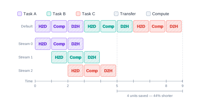
By default, every CuPy operation is submitted to the default stream. You can access the current stream as:
The default stream serializes operations. If you want to overlap work, you can create your own streams:
Use Stream.use() as a context manager to direct
operations to a specific stream:
PYTHON
# Operations in stream1
with stream1.use():
    a = cupy.random.normal(size=1_000_000)
    b = cupy.random.normal(size=1_000_000)
    result1 = a + b

# Operations in stream2 (may run concurrently with stream1)
with stream2.use():
    c = cupy.random.normal(size=1_000_000)
    d = cupy.random.normal(size=1_000_000)
    result2 = c + d

# Synchronize both streams to wait for completion
stream1.synchronize()
stream2.synchronize()
From Python’s perspective, each step will appear to execute
immediately until we reach the calls to synchronize(),
which will block. In reality, what we’ve done is to queue up these
operations into each of stream1 and stream2,
which (may) execute their operations concurrently.
Importantly: notice how we group together the data dependencies for
each sequence within the same stream. For example, notice that
arrays a and b are created in the same stream
where they are later used. (If we had data dependencies between
streams we would need to carefully and judiciously add calls to
synchronize().)
The key semantics are:
- Within a stream: operations are guanteed to execute in submission order.
- Between streams: operations may execute concurrently—the GPU schedules them based on available resources.
-
Synchronization: call
stream.synchronize()to block the CPU until all operations in that stream have completed.
A common idiom when using streams is to use them in combination with Python threads, where each Python thread has an associated default stream. If you’re already comfortable with Python threading, this can often simplify managing state.
To do this we must start Python with the environment variable
CUPY_CUDA_PER_THREAD_DEFAULT_STREAM=1. Then each Python
thread will, by default, dispatch operations to its own stream. For
example:
PYTHON
from concurrent.futures import ThreadPoolExecutor

def compute(c):
    # Each thread implicity uses its own stream on the GPU
    a = cupy.random.normal(size=1_000_000)
    b = cupy.random.normal(size=1_000_000)
    return c * (a + b)

with ThreadPoolExecutor as executor:
    results = executor.map(compute, [1, 2, 3, 4, 5])
Challenge
Create three arrays on the GPU, then perform three independent
computations (e.g., a * 2, b ** 2,
cupy.sin(c)) each in their own respective stream.
Synchronize all three streams and verify that the results are
correct.
PYTHON
s1 = cupy.cuda.Stream()
s2 = cupy.cuda.Stream()
s3 = cupy.cuda.Stream()

with s1.use():
    a = cupy.random.normal(size=1_000_000)
    r1 = a * 2

with s2.use():
    b = cupy.random.normal(size=1_000_000)
    r2 = b ** 2

with s3.use():
    c = cupy.random.normal(size=1_000_000)
    r3 = cupy.sin(c)

s1.synchronize()
s2.synchronize()
s3.synchronize()

# Verify
cupy.testing.assert_allclose(r1, a * 2)
cupy.testing.assert_allclose(r2, b ** 2)
cupy.testing.assert_allclose(r3, cupy.sin(c))
Advanced topic: Device selection
Many systems have multiple GPUs available, especially in supercomputing environments. To make full use of your allocation you need to be able to dispatch work across these GPUs.
Each GPU is fully independent: each has its own memory, its own streams, and its own computational availability. This degree of independence means that it is usually best to distribute work to GPUs that is similarly independent.
GPU selection can be done in varying levels of granularity:
-
Selecting the GPU prior to running the program: The
environment variable
CUDA_VISIBLE_DEVICEScan be used at program startup to filter which devices can be seen by the program. For example, a program started asCUDA_VISIBLE_DEVICES=2 python program.pywill only be able to see GPU device 2 and will default to using this device. -
Setting a default GPU from within the program: CuPy
will always set a default GPU which you can view as
cupy.cuda.Device(). You can view the number of available GPUs by callingcupy.cuda.runtime.getDeviceCount(), and the default can be changed at any point by callingcupy.setDevice(idx). - Dispatching data and operations to different GPUs on an adhoc basis.
For adhoc GPU device selection you can choose to either nominate the device for each call or use the device a context manager (similar to streams):
PYTHON
# Option 1: Manually nominate the destination GPU
a_d2 = cupy.array([1, 2, 3], device=2)
b_d2 = cupy.array([4, 5, 6], device=2)

# Both arrays _must_ exist on the same device before performing a computation
result = a_d2 + b_d2

# Option 2: use a context manager
with cupy.cuda.Device(3):
    arr = cupy.array([1, 2, 3])
    print(arr.device)  # <CUDA Device 3>
Challenge
Write code that discovers how many GPUs are available in the system, then creates a small array on each device and prints its device ID.
Content from Writing your first GPU kernels
Last updated on 2026-07-15 | Edit this page
Overview
Questions
- How does a single function body know which piece of data to process when launched thousands of times?
- How do you configure a kernel launch so every element of an array is covered, regardless of its size?
- How can threads safely combine their results into a single value?
Objectives
- Write and launch a GPU kernel with
@cuda.jit, configuring grid dimensions with appropriate block and thread counts. - Use the grid-stride loop pattern so kernels handle arrays of any size.
- Map a single thread index to multi-dimensional array coordinates.
- Implement a parallel reduction using shared memory, thread synchronisation, and atomic operations.
There are a few options for writing kernels in Python, however in this workshop we will prefer to use Numba. The reason for this is simple: Numba lets you write GPU kernels in (a limited subset of) Python. You will be able to draw on your existing knowledge of Python, and your existing tools, linters and syntax highlighting will all continue to work.
CuPy also makes it possible to write kernels, however the kernels are written in C and stored as text strings inside your python code; this means you must not only be proficient in C but you will also lose the syntax highlighting of your editor.
Whatever you choose, besides some syntactical differences, the concepts learned here translate one-to-one to kernels written directly in C or C++.
What is a kernel?
Let’s return to the example of adding two vectors elementwise. As a simple loop this looks like:
PYTHON
def adder(xs, ys, zs):
    for i in range(len(xs)):
        zs[i] = xs[i] + ys[i]

xs = np.random.normal(size=1000)
ys = np.random.normal(size=1000)
zs = np.empty_like(xs)
adder(xs, ys, zs)
This is an ideal candidate for data parallelism, since each iteration of the loop is independent.
In a parallel context, the interior of the loop is referred to as a
kernel. The kernel is a function that is called repeatedly and
identically for each parallel iteration. A kernel depends on one key bit
of information: the index i. This index tells the kernel
“where” it is, and in this case which part of the input and output
vectors are its concern.
For clarity, let’s rewrite this as a parallel loop and with the kernel as a stand alone function:
PYTHON
@njit
def kernel(i, xs, ys, zs):
    zs[i] = xs[i] + ys[i]

@njit(parallel=True)
def adder(xs, ys, zs):
    for i in prange(len(xs)):
        kernel(i, xs, ys, zs)

N = 1000
xs = np.random.normal(size=N)
ys = np.random.normal(size=N)
zs = np.empty_like(xs)
adder(xs, ys, zs)
Remember: @njit compiles the function it wraps to
machine code that runs directly on the CPU.
In GPU programming, your work will be all about writing the kernel itself. The outer loop, on the other hand, is something that the GPU will manage for you. It is up to the GPU to decide how to parallelise that loop, when to run the kernels, and the order they execute in.
A first kernel
Let’s try writing this adder function as a kernel on the GPU.
PYTHON
import math
import numpy as np
import cupy
from numba import cuda

@cuda.jit
def adder_gpu(xs, ys, zs):
    i = cuda.grid(1)
    if i < len(xs):
        zs[i] = xs[i] + ys[i]

N = 1000
xs_d = cupy.random.normal(size=1000)
ys_d = cupy.random.normal(size=1000)
zs_d = cupy.empty_like(xs_d)

nthreads = 256
nblocks = math.ceil(N / nthreads)
adder_gpu[nblocks, nthreads](xs_d, ys_d, zs_d)
There’s a lot to unpack in this brief snippet of code:
- First, we added a new import:
from numba import cuda. -
We’ve wrapped our kernel with the decorator
@cuda.jit. Just like@numba.jit, this will allow the kernel to compile “just in time” (jit) when we call it based on the input types (e.g. the types ofxs,ys, andzs). The difference is@numba.jitcompiled this kernel for the CPU, whereas@cuda.jitis compiled for the GPU. There is an overhead associated with this initial compilation but subsequent calls will re-use the cached kernel so long as the input types remain unchanged. -
We’ve called
cuda.grid(1)to determine the index of the kernel. Unlike our previous example, the index is not passed in as an argument. We’ve also added a condition to check the index is within range. -
We’ve allocated our GPU arrays using
cupy.array(). CuPy GPU arrays are compatible withnumba.cudakernels. Numba provides its own methods too, such ascuda.device_array(),cuda.to_device()andarray_d.copy_to_host(), and you might want to use these instead if you don’t want CuPy as a dependency in your project. -
We’ve called the
adder_gpu()function by first providing grid dimensions: blocks and threads per block. Grid dimensions configure how many times the kernel is run and are directly related to the kernel’s index. Each time you call a GPU kernel, you must configure its grid dimensions. We will discuss grid configuration in depth shortly. - All array and memory allocations occur outside of the kernel. The kernel cannot allocate global memory and so these arrays must be passed as arguments.
-
The kernel does not return anything (or implicitly, returns
None). Kernels do not return values, and their “outputs” must
be provided as a mutable input. In this case, the output is
zswhich must be allocated outside the kernel and passed as an argument to the kernel.
Challenge
Try benchmarking each of the parallel CPU and GPU adder functions. Which is faster? Try making N larger: is there a point where their respective speeds swaps?
PYTHON
@njit
def kernel(i, xs, ys, zs):
    zs[i] = xs[i] + ys[i]

@njit(parallel=True)
def adder(xs, ys, zs):
    for i in prange(len(xs)):
        kernel(i, xs, ys, zs)

@cuda.jit
def adder_gpu(xs, ys, zs):
    i = cuda.grid(1)
    if i < len(xs):
        zs[i] = xs[i] + ys[i]

N = 12_000_000

xs = np.random.normal(size=N)
ys = np.random.normal(size=N)
zs = np.empty_like(xs)

xs_d = cupy.array(xs)
ys_d = cupy.array(ys)
zs_d = cupy.empty_like(xs_d)

result = cupyx.profiler.benchmark(lambda: adder(xs, ys, zs), n_repeat=100)
print(result)

nthreads = 256
nblocks = math.ceil(N / nthreads)
result = cupyx.profiler.benchmark(lambda: adder_gpu[nblocks, nthreads](xs_d, ys_d, zs_d), n_repeat=100)
print(result)
On my machine, the CPU remains faster for all workloads where N < 10,000,000 values. At around about 12,000,000 values, the CPU version begins to rapidly increase in duration and to be less performant than the GPU.
(Bonus question: why do you think the CPU version suddenly reaches a performance cliff?)
Grid dimensions
Recall that the GPU is responsible for managing the parallelisation of our kernels. It’s up to us, however, to configure how that parallelisation occurs and in the CUDA model this occurs by setting the grid dimensions.
A grid is composed of one or more thread blocks, each with a fixed number of threads. The total number of threads in a grid is the number of thread blocks multiplied by the number of threads.
When a kernel is run, the work is distributed in the following manner:
- The GPU scheduler parcels off thread blocks, and enqueues it to each streaming multiprocessor (SM) as it has some availability.
- Each SM is then, in turn, responsible for scheduling the thread block to run as a series of warps (32 or 64 threads that run in lockstep) as soon as it has idle cores.
You might wonder at this point: threads make sense as they’re the fundamental unit of parallelisation, but why do I need to group them into blocks? And the answer is linked to the hardware design of the GPU. Inter-thread coordination, synchronisation and communication can only occur within a SM, which in turn means only within a thread block. So far we’ve seen kernel examples that don’t require these facilities, but many workloads (and optimisations) need inter-thread coordination or communication.
There’s a few things to factor in when choosing a grid size:
- Ideally, choose the number of threads per block to be a multiple of your warp size. This means multiples of 32 threads for NVIDIA hardware and 64 for AMD. Remember that threads are executed in lockstep as a warp; if its not a round multiple, any excess cores will nonetheless be enrolled in the warp with their result ignored.
- Don’t make the threads per block too large. You want to strike a balance where you have a lot of blocks so that each SM has a queue of work that it can cycle through as its cores become idle; at the same time you want to ensure the blocks are large enough to mitigate overheads from block scheduling.
- Rarely will a grid size match the problem size. Whilst your threads per block must be a multiple of 32, we wouldn’t expect your data to also be an even multiple. When sizing your grid, you’ll need to ensure your kernel includes a condition that checks that its index lies within the data.
A good rule of thumb for threads per block is somewhere between 128 to 1024 threads. As always benchmark your code.
Your grid can be 1, 2, or 3 dimensional. As an example, if we were adding two large matrices we might choose to index by row and column. In this case our code might look like:
PYTHON
@cuda.jit
def adder(xs, ys, zs):
    i, j = cuda.grid(2)  # The argument to grid determines the dimension of the grid

    if i < xs.shape[0] and j < xs.shape[1]:
        zs[i, j] = xs[i, j] + ys[i, j]

xs = cupy.random.normal(size=(8192, 8192))
ys = cupy.random.normal(size=(8192, 8192))
zs = cupy.empty_like(xs)

adder[(256, 256), (32, 32)](xs, ys, zs)
In practice, it is more common to use a one dimensional index.
In actual fact, cuda.grid() and its sibling
cuda.gridsize() (which returns the total number of threads
across the grid) are helper functions. They wraps the more primitive
variables:
-
cuda.threadIdx.x: the thread index within the thread block -
cuda.blockDim.x: the number of threads per block -
cuda.blockIdx.x: the block index within the grid -
cuda.gridDim.x: the number of blocks in the grid
(For multidimensional grids, the additional indices are available at
.y and .z,
e.g. cuda.threadIdx.y.)
Based on this, we can write our own versions of the helper functions:
-
cuda.grid(1)is equivalent tocuda.blockIdx.x * cuda.blockDim.x + cuda.threadIdx.x -
cuda.gridsize(1)is equivalent tocuda.blockDim.x * cuda.gridDim.x
You should be comfortable with both versions as you’ll see them used interchangably. Additionally, the extra information about where a thread lies within its block will prove useful in later kernels.
Challenge
Return to adder_gpu (with 1D grid) and modify the code
so that it ensures the full arrays are added irrespective of
the grid size. That is, ensure the each element is added whether the
grid is sized too small or too large.
Hint: try replacing the if condition with a
for loop having a step size given by
cuda.gridsize(1).
With the new configuration try modifying the thread and block count:
- What happens to the performance if you set the thread blocks to 1 and threads per block to 256? Why?
- What happens if you set
nthreadsvery large, perhaps to 4096?
Using a for loop like this is a very common idiom in kernel design, known as a grid stride loop. As before, it ensures we stay within the bounds of the array, but it doesn’t rely on the grid being at least as large as the problem. Later, you’ll see it lends itself to other common optimisations.
When the block size is set to 1, the GPU is able to utilise only one of its SMs. The rest will sit idle, resulting in very poor utilisation of the GPU, also known as occupancy.
When the thread size is too large, your kernel may crash. When especially large, the kernel may exceed the shared resources of the SM, for example its register space. It’s rare that thread counts greater than 1024 are useful or performant.
Challenge
Rewrite the adder kernel using the underlying thread and block
indices directly, instead of grid() and
gridsize.
An aside: warp divergence
We’ve talked earlier about how a warp executes its threads in
lockstep. But in the previous examples we included the condition
cuda.grid(1) < len(xs). How can a SIMT execution model
handle a condition?
When a warp encounters a condition, it will first evaluate the condition. Then:
- If the condition evaluates identically across the warp (e.g. each thread evaluates to true), then the warp will continue executing the one conditional branch.
- On the other hand, if threads evaluate differently across the warp then we get warp divergence. In this case, the warp must evaluate both branches of the condition, and due to the lockstep nature of SIMT, it will do this sequentially: first one branch, and then the other. Each thread that is not part of the current conditional branch will be masked, essentially performing a “no-op” for each of their respective processor cycles.
Warp divergence is expensive since it wastes processor cycles. You will want to ensure warp divergence occurs in as few warps as possible, and this plays a factor in both kernel design and grid configuration.
In the previous adder kernel, you will notice warp
divergence occurs in exactly one warp: the warp whose index range
breaches the length of the underlying arrays.
Multiplier
Challenge
With just minor modifications, change the 1D adder_gpu
kernel to a multiplier kernel that computes elementwise
multiplication. e.g. \(z_i = x_i \times
y_i\). Use the grid stride loop pattern.
Also add a test to ensure correctness.
PYTHON
@cuda.jit
def multiplier(xs, ys, zs):
    for i in range(cuda.grid(1), len(xs), cuda.gridsize(1)):
        zs[i] = xs[i] * ys[i]

N = 12_000_000
xs_d = cupy.random.normal(size=N)
ys_d = cupy.random.normal(size=N)
zs_d = cupy.empty_like(xs_d)

nthreads = 256
nblocks = math.ceil(N / nthreads)
multiplier[nblocks, nthreads](xs_d, ys_d, zs_d)

cupy.testing.assert_allclose(zs_d, xs_d * ys_d)
Matrix multiplication
Let’s attempt to write our own kernel that performs matrix multiplication. Recall that if \(A\) is an \(m \times n\) matrix, and \(B\) a \(n \times p\) matrix, then their product is a \(m \times p\) matrix \(C\) having elements \(c_{ij} = \sum_{k=1}^n a_{ik} b_{kj}\).
Let’s begin by first writing this in simple Python as a series of for loops:
PYTHON
def matmul(A, B, C):
    for i in range(C.shape[0]):
        for j in range(C.shape[1]):
            for k in range(A.shape[1]):
                C[i, j] += A[i, k] * B[k, j]

A = np.random.normal(size=(32, 16))
B = np.random.normal(size=(16, 24))
C = np.zeros((32, 24))
matmul(A, B, C)

np.testing.assert_allclose(C, A @ B)
When considering how to design a kernel for this problem, we need to answer a few interrelated questions:
- What is a unit of parallelisation? Or put differently, what does the index of each kernel map to in our problem domain? Is it an element in one (or both) of the input matrices? Is it an element of the output matrix? Is it a row or column?
- How should we configure our grid? What is the span of the grid and what is its dimension?
Challenge
Consider the following four variants of kernels and associated grid configurations. Which is the preferred choice and why?
PYTHON
# Grid: 3D grid over all values of i, j, k
def kernel1(i, j, k, A, B , C):
    C[i, j] += A[i, k] * B[k, j]

# Grid: 2D grid over all values of i, j
def kernel2(i, j, A, B, C):
    for k in range(A.shape[1]):
        C[i, j] += A[i, k] * B[k, j]

# Grid: 2D grid over all values of i, k
def kernel3(i, k, A, B, C):
    for j in range(C.shape[1]):
        C[i, j] += A[i, k] * B[k, j]

# Grid: 1D grid over all values of i
def kernel4(i, A, B, C):
    for j in range(C.shape[1]):
        for k in range(A.shape[1]):
C[i, j] += A[i, k] * B[k, j]Two considerations stand out when comparing the kernel options:
-
Race conditions: Recall that reading, computing,
and writing to memory in parallel code does not happen all at once, and
multiple threads competing to do this to the same memory
location will introduce race conditions. Kernels 1 and 3
both introduce kernels with race conditions. In kernel 1, for each
i,jcoordinate there will bekcompeting kernels. The situation is similar for kernel 3. There are (complex) ways to mitigate these race conditions but we would have to be justified in taking this route. - Maximal parallelisation: All things being equal, we would typically want to maximise the degree of parallelisation and fan out the work across the many thousands of cores of the GPU. Kernel 1 has \(i \times j \times k\) threads which, if it didn’t suffer from race conditions, would be ideal. In contrast, kernel 4 parallelises only over the \(i\) rows of \(A\) and for most sizes of matrices even with thousands of rows, this will result in poor GPU occupancy. Kernel 2, on the other hand, has \(i \times j\) threads, which even for kernels with dimensions of only a few hundred rows and columns results in tens of thousands of threads.
On these grounds, kernel 2 is the preferred option with a 2D grid configuration that spans \(i \times j\).
Challenge
Have a go at filling in the missing lines from within the kernel definition and grid configuration.
PYTHON
@cuda.jit
def matmul(A, B, C):
    i, j = cuda.grid(2)
    if i < C.shape[0] and j < C.shape[1]:
        # TODO

A = cupy.random.normal(size=(100, 200))
B = cupy.random.normal(size=(200, 150))
C = cupy.zeros((100, 150))

threads = 16
nblockx = math.ceil( #TODO )
nblocky = math.ceil( #TODO )
matmul[(nblockx, nblocky), (threads, threads)](A, B, C)

cupy.testing.assert_allclose(C, A @ B)One solution looks like this:
PYTHON
@cuda.jit
def matmul(A, B, C):
    i, j = cuda.grid(2)
    if i < C.shape[0] and j < C.shape[1]:
        for k in range(A.shape[1]):
            C[i, j] += A[i, k] * B[k, j]
And with the following grid configuration:
PYTHON
threads = 16
nblockx = math.ceil(C.shape[0] / threads)
nblocky = math.ceil(C.shape[1] / threads)
matmul[(nblockx, nblocky), (threads, threads)](A, B, C)
An alternative is to store the partial sum in a local
variable before writing out to the global memory location at
C[i, j]. For example:
PYTHON
@cuda.jit
def matmul(A, B, C):
    i, j = cuda.grid(2)
    if i < C.shape[0] and j < C.shape[1]:
        cij = 0.0
        for k in range(A.shape[1]):
            cij += A[i, k] * B[k, j]

        C[i, j] = cij
Try benchmarking these two versions. Which is faster? Can you guess why?
Challenge
Rewrite the matrix multiplication using a 1D grid. Under this
configuration, every kernel is still responsible for a single element of
\(C\) but it must map from a 1D index
to a 2D index. What is the span of the 1D grid? Hint: familiarise
yourself with the Python function divmod().
PYTHON
@cuda.jit
def matmul(A, B, C):
    ij = cuda.grid(1)

    if ij < C.size:
        i, j = divmod(ij, C.shape[1])

        for k in range(A.shape[1]):
            C[i, j] += A[i, k] * B[k, j]


A = cupy.random.normal(size=(100, 200))
B = cupy.random.normal(size=(200, 150))
C = cupy.zeros((100, 150))

threads = 256
nblocks = math.ceil(C.size / threads)
matmul[nblocks, threads](A, B, C)

cupy.testing.assert_allclose(C, A @ B)
Discrete Fourier transform
We’ve previously used broadcasting to perform a discrete Fourier transform (DFT). In this section we will guide you through writing your own from scratch.
For simplicity, we’ll consider just a one-dimensional transform which is defined as:
\(X_k = \sum_n^N x_n e^{-2 i \pi \frac{k n}{N}}\)
In all the examples, we’ll be using a complex input given by:
for varying values of N.
Part 1
Write the DFT using a simple python for loop. At this
stage, set N to be small (~100).
Check your routine by comparing the answer to numpy’s own FFT.
Part 2
Parallelise your code on the CPU using numba’s prange
function and njit decorator. Which loop or loops are
parallel? What is the unit of parallelisation?
Extract the inner loop as a standalone kernel function.
We parallelise over \(k\) but not \(n\), since including \(n\) would introduce race conditions.
Part 3
Complete the transition to a working GPU kernel:
- Modify your kernel into a GPU kernel by using the decorator
cuda.jitand by retrieving the index usingcuda.grid(1). (Don’t forget to add a condition that checks bounds!) - Minimise writes to global memory in your kernel by using a local accumulator variable.
- Configure a 1D grid using 256 threads and calculate the number of required blocks.
- Ensure the input and output arrays reside on the GPU.
By the end, you should have a working GPU kernel. Check that the
kernel works correctly by comparing to cupy.fft.fft().
Hint: Complex exponentials
(e.g. np.exp(1j * phase)) are not directly available inside
Numba CUDA kernels. The trick is to recall that \(e^{i \theta} = \cos{\theta} + i
\sin{\theta}\) and to use this identity with
math.cos() and math.sin() (which are available
for real values). That is: replace np.exp(1j * phase) with
complex(math.cos(phase), math.sin(phase)). Don’t forget to
import math at the top of your file.
PYTHON
@cuda.jit
def dft(xs, Xs):
    k = cuda.grid(1)
    N = len(xs)

    if k < N:
        xs_k = complex(0)
        for n in range(N):
            phase = -2 * np.pi * k * n / N
            xs_k += xs[n] * complex(math.cos(phase), math.sin(phase))

        Xs[k] = xs_k

N = 100_000
xs = cupy.random.normal(size=N) + 1j * cupy.random.normal(size=N)
Xs = cupy.zeros_like(xs)

threads = 256
nblocks = math.ceil(N / threads)

dft[nblocks, threads](xs, Xs)

cupy.testing.assert_allclose(Xs, cupy.fft.fft(xs))
Advanced topic: Parallel reductions
A reduction is
an operation that combines multiple elements down to one. Think, for
example, summing an array where the reduction operator is addition
(+). Often times the input array will be modified first
(known as a map) and then reduced, with the combined operation known as
a mapreduce.
In parallel contexts, reductions are not easy to write. Consider the following implementation of a sum:
PYTHON
@cuda.jit
def sum(xs, acc):
    # Each thread performs a partial sum
    _acc = 0
    for i in range(cuda.grid(1), len(xs), cuda.gridsize(1)):
        _acc += xs[i]

    acc[0] += _acc

N = 100_000_000
xs = cupy.random.normal(size=N)
acc = cupy.zeros(1)

threads = 256
nblocks = math.ceil(N / threads / 4)  # each thread will add 4 elements of xs
sum[nblocks, threads](xs, acc)
In general, this will fail. Can you see why?
As we saw in the parallelism section, this fails due to a race condition: each thread is attempting to read, add, and write a value to global memory, walking all over each other.
One tool in our toolbox are atomic
operations. These are a limited set of operations (e.g. +,
max, min, but not multiplication!) on a
limited set of types (mostly just floats and integers) that allow us to
do something like a read-add-write as a single operation. In
this case, we can use cuda.atomic.add() and see how this
works:
PYTHON
@cuda.jit
def sum(xs, acc):
    # Each thread performs a partial sum
    _acc = 0
    for i in range(cuda.grid(1), len(xs), cuda.gridsize(1)):
        _acc += xs[i]

    cuda.atomic.add(acc, 0, _acc)
The tests pass, meaning that this is at least correct. But if we benchmark you’ll see that it is very slow. And the simple reason is that atomic operations don’t come for free. It still ultimately forces some kind of serialisation of the operations.
The idiomatic solution to a reduction is twofold: perform a reduction within a thread block, followed by a reduction across the full grid.
To do this, we’re going to introduce shared memory: shared memory is memory that is visible by each member of a thread block. The general idea is this:
- Each thread will perform a local, partial sum.
- We will construct a shared memory array that has a size that exactly matches the threads per block.
- Each thread in a thread block will set its associated entry in the shared array to its partial sum.
- The thread block will sum the contents of its shared memory using a binary reduction (see diagram).
- Finally, thread ID=0 of the thread block will perform an atomic add to global memory.
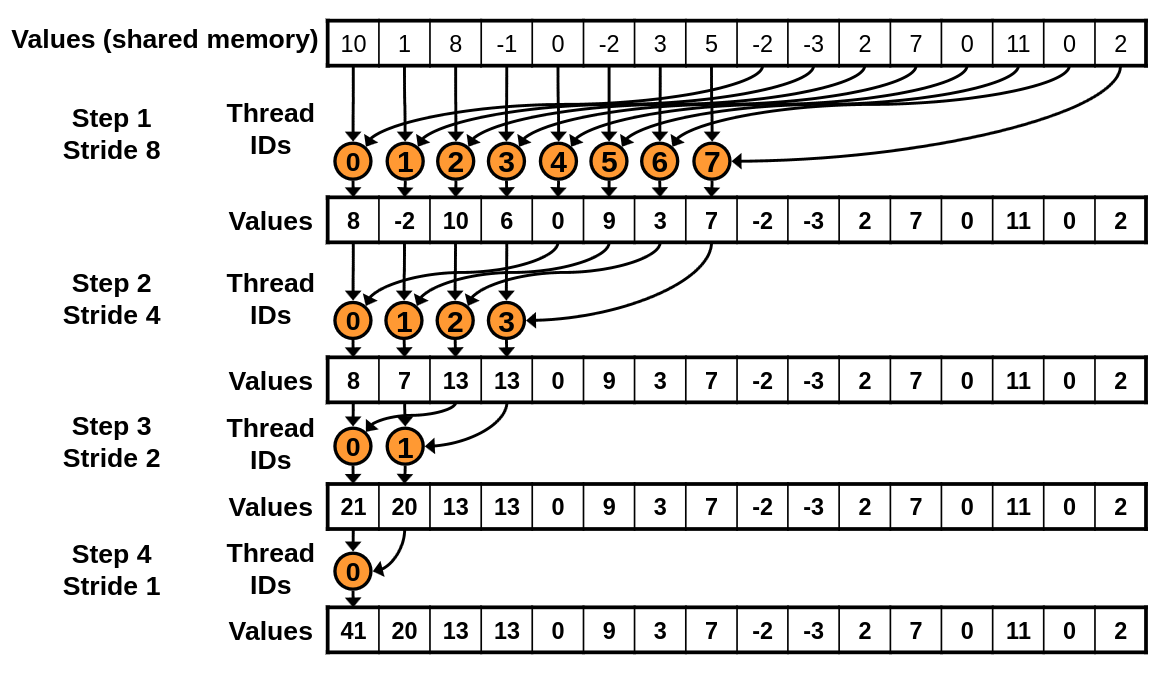
Caption: An illustration of a binary reduction within thread block. On each step, only half the number of threads participate in the reduction as in the previous step. [Source]
One such implementation looks like this:
PYTHON
@cuda.jit
def sum(xs, acc):
    # Allocate a shared array sized to match the threads per block
    shared = cuda.shared.array(256, dtype=np.float64)

    # Each thread performs a partial sum
    _acc = float(0)
    for i in range(cuda.grid(1), len(xs), cuda.gridsize(1)):
        _acc += xs[i]

    # Every thread loads its partial sum into its associated shared memory address
    tid = cuda.threadIdx.x  # thread ID - not grid ID!
    shared[tid] = _acc

    # Reduction of the shared memory across the thread block
    for offset in (128, 64, 32, 16, 8, 4, 2, 1):
        cuda.syncthreads()
        if tid < offset:
            shared[tid] += shared[tid + offset]

    # Thread ID=0 adds the entire thread block sum to global memory
    if tid == 0:
        cuda.atomic.add(acc, 0, shared[0])
Notice the use of cuda.syncthreads(): this is a
synchronisation method that ensures all threads in a thread block have
reached this point. (Remember that only warps execute in lockstep.) This
is necessary once we start interacting with shared memory, since we need
to guarantee that the entirety of the thread block has fully written to
its shared memory address before any thread tries to make a read.
Benchmarking shows this function is now quite fast. The cost of the
atomic add is now mitigated by the fact that it is called only once for
every thread block. For large arrays, this function is almost as fast as
the highly optimised cupy.sum().
For more information about advanced reduction optimisations including
use warp intrinsics, I recommend these NVIDIA
slides.
Content from Optimisation
Last updated on 2026-07-22 | Edit this page
Overview
Questions
- Why is accessing global memory in a kernel’s hot loop a performance bottleneck?
- How can threads within a block cooperate to share the cost of reading data from global memory?
- When does using lower-precision floating point numbers make your kernel faster?
Objectives
- Recognise when a kernel is memory-bound versus compute-bound and apply targeted optimisations.
- Reduce global memory traffic by caching data in shared memory and coalescing memory accesses.
- Choose appropriate floating-point precision and use specialised CUDA math functions to improve throughput.
- Explain the trade-offs of thread coarsening: fewer thread blocks in exchange for higher computational intensity per thread.
A toy problem
We’re going to start with a toy problem: imaging radio interferometry data. In other domains, this is also known as a non-uniform Fourier transform: we transform from an irregularly sampled 3D visibility space to a 2D surface within the imaging space.
An important non-aim: we are not looking to make algorithmic improvements. Real-world imaging software rarely performs a full direct Fourier transform since it is so costly, but those alternative algorithms are more complex and are not our focus here.
The discrete imaging equation is defined as follows:
\[ V(l, m) = \sum V(u, v, w) e^{2 \pi i (u l + v m + w [n - 1])} \\ \textrm{where} \quad n = \sqrt{1 - l^2 - m^2} \]
The dimensions \(l\) and \(m\) span the image domain, whilst the \(u, v, w\) coordinates span the (sparse and unevenly sampled) visibility domain. We are prohibited from treating this as a simple 2D fast Fourier transform problem due to two main factors: u, v, w are not even sampled; and the so-called \(w\) term is non-negligible.
Image sizes are typically thousands of pixels by thousands of pixels; whilst visibility data is similarly millions of rows in length.
By the end, we hope to be able to image the large radio lobes of Fornax A from the raw visibility data.

A first implementation
As always, we will approach this first on the CPU where we can ensure we first make things right before attempting a first pass at a kernel.
Let’s first set things up. Our data is stored in the file visibilities.npz
which is also available at
/fred/oz983/gpu-workshop/visibilities.npz on the OzStar
system. We will extract each datum and its associated baseline
coordinates:
PYTHON
data = np.load("/fred/oz983/gpu-workshop/visibilities.npz")
us, vs, ws, vis = data["u"], data["v"], data["w"], data["data"]
Next we will set up our imaging grid. We will image a 700 x 700 pixel grid. We will set the scale such that \(\Delta l = \Delta m = 10^{-4}\) (this scale is somewhat arbitrary but is chosen to match the main radio feature within the image).
Finally, we will precompute the associated values \(n' = n - 1 = \sqrt{1 - l^2 - m^2} - 1\):
Challenge
Using numba’s njit and prange functions,
attempt to write an CPU-parallel implementation of the direct imaging
equation. Ask yourself: what is the unit of parallelisation?
Using matplotlib’s imshow(), save a figure of the real
components of the image.
Note: below we reduce the data by 50x to speed things up. If things take too long for you, try reducing the data even more aggressively.
PYTHON
@njit(parallel=True)
def image_numba(us, vs, ws, vis, ls, ms, ndashes, img):
pass
# TODO
data = np.load("/fred/oz983/gpu-workshop/visibilities.npz")
us, vs, ws, vis = data["u"], data["v"], data["w"], data["data"]
lpx, mpx = np.mgrid[-350:350, -350:350]
ls, ms = lpx * 0.0005, mpx * 0.0005
ndashes = np.sqrt(1 - ls**2 - ms**2) - 1
# For now, reduce data by 50x since CPU is too slow
us, vs, ws, vis = us[::50], vs[::50], ws[::50], vis[::50]
img = np.zeros(ls.shape, dtype=complex)
image_numba(us, vs, ws, vis, ls, ms, ndashes, img)
plt.imshow(img.real, origin="lower")
plt.savefig("output.png")We parallelise over each pixel which, for a 700 x 700 pixel image, gives us just shy of 500,000 threads. And since each pixel is its own independent sum, we don’t have to worry about race conditions.
PYTHON
@njit(parallel=True)
def image_numba(us, vs, ws, vis, ls, ms, ndashes, img):
    # Parallelise over each output pixel
    for lmpx in prange(ls.size):
        # Convert 1D to 2D pixel index
        lpx, mpx = lmpx // ls.shape[1], lmpx % ls.shape[1]

        # Retrieve l, m and ndash coordinates associated with this pixel
        l, m, ndash = ls[lpx, mpx], ms[lpx, mpx], ndashes[lpx, mpx]

        # Perform the sum for this one pixel over all of the visibility data
        for u, v, w, datum in zip(us, vs, ws, vis):
            phase = 2 * np.pi * (u * l + v * m + w * ndash)
            img[lpx, mpx] += datum * np.exp(1j * phase)
Even with only a fifthieth of the data we start to see something resembling the radio lobes:
Challenge
Now that we have a working CPU version, the next step is to extract the inner loop as a standalone kernel and configure an associated grid to work on the GPU.
Try implementing a simple GPU kernel implementation using the
@cuda.jit decorator.
Note: As with the DFT function we have worked on earlier, you will need to rewrite the imaginary exponential using the identity \(e^{i \phi} = \cos{\phi} + i \sin{\phi}\).
The implementation is very similar to that used in Numba’s prange loop. Some points of note:
- We have chosen here to retain a linear index for simplicity. Additionally, in the case where the image dimensions don’t match an even multiple of the threads per block, the 1D grid minimises the amount of threads that “overflow”.
- We have rewritten the imaginary exponential as a combination of
cos()andsin().
PYTHON
@cuda.jit
def kernel(us, vs, ws, vis, ls, ms, ndashes, img):
    lmpx = cuda.grid(1)

    if lmpx < img.size:
        lpx, mpx = divmod(lmpx, ls.shape[1])

        # Retrieve l, m and ndash coordinates associated with this pixel
        l, m, ndash = ls[lpx, mpx], ms[lpx, mpx], ndashes[lpx, mpx]

        # Perform sum over all of the visibility data for just one pixel
        for u, v, w, datum in zip(us, vs, ws, vis):
            phase = 2 * np.pi * (u * l + v * m + w * ndash)
            img[lpx, mpx] += datum * complex(math.cos(phase), math.sin(phase))
We can benchmark this code using the following harness:
PYTHON
# Load the visibility data
data = np.load("/fred/oz983/gpu-workshop/visibilities.npz")
us, vs, ws, vis = data["u"], data["v"], data["w"], data["data"]

# Initialise the image grid and the corresponding l, m and ndash coordinates
lpx, mpx = np.mgrid[-350:350, -350:350]
ls, ms = lpx * 0.0005, mpx * 0.0005
ndashes = np.sqrt(1 - ls**2 - ms**2) - 1

# Transfer data to the GPU
img_d = cupy.zeros(ls.shape, dtype=complex)
us_d, vs_d, ws_d, vis_d, ls_d, ms_d, ndashes_d = map(
    cupy.array, [us, vs, ws, vis, ls, ms, ndashes]
)

nthreads = 256
nblocks = math.ceil(img_d.size / nthreads)

result = cupyx.profiler.benchmark(
    lambda: kernel[nblocks, nthreads](
        us_d, vs_d, ws_d, vis_d, ls_d, ms_d, ndashes_d, img_d
    ),
    n_repeat=3,
    n_warmup=1,
)
On my machine, this first kernel is fast enough to allow us to image the full set of data giving a lovely image of Fornax A:
Do you think it would be possible to write this kernel using CuPy’s array-level operations and broadcasting rules? What kind of challenges might you encounter and how could they be mitigated?
Like with the DFT, this would be two-fold operation: a broadcasting operation that would produce a 3-dimensional array, following by a reduction along one axis. The sheer amount of data would mean this would not fit in memory. Some mitigations include:
- Batching the data by repeatedly processing bounded chunks of the input data that will fit in memory
- Or alternatively, processing all input data but for a limited number of pixels at a time, and iterating over the full image from in Python
An aside: Profiling with NSIGHT
Up till now we have used simple timers to measure performance. NVIDIA provides an alternative, extremely detailed set of benchmarking tools:
- NSIGHT Compute: Provides detailed analysis of a kernel, including its register usage, FMA instruction counts, memory accesses, and so on. This is most useful when optimising a specific kernel.
- NSIGHT Systems: A higher-level profiler that can show a timeline of memory transfers, kernel runtimes, streams, and the interleaved dependencies between these different GPU processes. This is most useful to understand the full lifecycle of a program and to help prioritise optimisation work.
In my personal experience, NSIGHT Systems can be very useful to understand how your program runs, how kernels might be delayed by dependencies such as memory transfers, and how this might be mitigated by using multiple CUDA streams.
Our task here, however, is purely in optimising the kernel itself, and this is specifically the role for NSIGHT Compute. Unfortunately, I have rarely found this to be useful tool. NSIGHT Compute tabulates all sorts of hardware counters (FMA instructions, cache hits, memory accesses, etc.) which by itself is overwhelming and rarely useful to the non-expert. Along with this raw data, it also tries to formulate suggestions as to how to improve your kernel; I’ve found these suggestions to be usually hit and miss.
Some things that NSIGHT Compute can be useful for are:
- Checking for precision: are there some accidental 64 bit precision operations in your kernel that is otherwise meant to be purely 32 bit precision?
- Understanding what is limiting you: are you compute bound or memory bound? Learn to interpret roofline plots.
- What is the ratio of fused multiply add (FMA) to total floating point instructions? Are you poorly using the more efficient FMA instruction?
Nonetheless, we will be proceeding without these tools and instead we will be presenting the standard set of optimisation techniques that apply to almost all kernel work. If you do use NSIGHT Compute in your work and it warns of poor occupancy, or non-coalesced memory accesses, after this section you will know what these warnings mean. Hopefully, you will also develop an intuition about whether its recommendations are worth pursuing or not.
Optimisation pitfalls
As with making the choice to rewrite an algorithm from a straightforward sequential implementation to a parallel implementation, the choice to optimise comes with some downsides that must be kept in mind.
From the outset you should understand the kind of performance that is necessary to make your original problem computationally tractable and optimise with this concrete goal in mind. Don’t optimise for the sake of optimisation.
As you will see as we progress here, optimisation comes with important downsides:
- It’s not always possible! Sometimes the “obvious” optimisations do very little at all, and despite the advertised computational performance of your hardware, these optimisation strategies fail to meaningfully close this gap. This may be because of hardware limits such as memory pressure, intractable aspects of your algorithm, or the unfortunate consequence of the black box that is an optimising compiler. Know when to raise the white flag.
- Optimisation almost invariably results in code bloat. Your code will become substantially longer and substantially more complex.
- Your code will become harder to reason about.
- And as a consequence, you may introduce bugs.
Optimisation 1: Minimise writing to global memory
We’ve already touched on this optimisation strategy before, but it’s important enough to repeat here: reading and writing to global memory is expensive and currently our kernel writes to global memory on every single inner loop.
Memory ordered from fastest to slowest is: local memory, then shared memory, and finally global memory. But by the same token, there is far less local and shared memory storage available; local arrays should typically be sized in the single digits, and shared arrays should typically be sized at most to a few hundred or so entries. (Large reservations of local and shared arrays cause a scarcity of memory and result in fewer simultaneous thread blocks being scheduled in a SM.)
How do you identify which memory is which?
-
Global memory is any array that is created on the
host side (e.g. via
cupy.array(...)) and passed as an argument to the kernel -
Shared memory is memory that is created inside the
kernel via
cuda.shared.array(...) -
Local memory are any scalar variables created
within the kernel as well as fixed-length arrays created using
cuda.local.array(...)
Challenge
Rewrite the kernel to use a local accumulator variable.
- Initialise a summation variable prior to the loop.
- On each innerloop iteration, append to this variable (using
+=). - Finally, write the value of this variable to global memory at the culmination of the kernel.
PYTHON
@cuda.jit
def kernel(us, vs, ws, vis, ls, ms, ndashes, img):
    lmpx = cuda.grid(1)

    if lmpx < img.size:
        lpx, mpx = divmod(lmpx, ls.shape[1])

        # Retrieve l, m and ndash coordinates associated with this pixel
        l, m, ndash = ls[lpx, mpx], ms[lpx, mpx], ndashes[lpx, mpx]

        # Perform sum over all of the visibility data for just one pixel
        pixel = complex(0)
        for u, v, w, datum in zip(us, vs, ws, vis):
            phase = 2 * np.pi * (u * l + v * m + w * ndash)
            pixel += datum * complex(math.cos(phase), math.sin(phase))

        img[lpx, mpx] = pixel
Optimisation 2: Floating point precision
You may be aware that floats come in different sizes, which correlate
to different precisions. In C, the standard options are
float and double, which correspond to 32 and
64 bit precision. CUDA provides a range of lower precision types such as
a 16 bit float (and even some non-standard numerical types that make
different trade offs between mantissa and exponent).
Unfortunately, Python hides the types of values and you may not be used to thinking about the precision of your calculations.
On the CPU, floating point performance usually doesn’t depend on the precision. That is, the performance ratio of 32 and 64 bit floats is 1:1 (with the important previso that 32 bit floats benefit from their smaller memory footprint). On the GPU, however, the performance ratio can vary enormously, and differs from one GPU to the next. For example, some AMD GPUs have a 1:1 performance ratio which is great for high precision numerical calculations; NVIDIA GPUs, on the other hand, strongly prefer lower precision floats, and this imbalance has increased considerably as their GPUs have been optimised towards AI workloads. A desktop NVIDIA 5080 card, for example, has a performance ratio of 1:64, and their recent datacenter B200 GPU has a performance ratio of 1:2:32 for 64/32/16 bit computations.
The upshot is: always compute at the minimal precision required.
To do this for our kernels, there are a few things we need to do:
Initialise all arrays by explicitly passing the optional
dtypekeyword argument and setting tonp.float64,np.float32,np.float16(or their complex equivalents,np.complex128andnp.complex64).Use the
dtypeattribute when transferring arrays to the GPU. For example,arr_d = cupy.array(arr, dtype=np.float32)will transfer and cast the floating point values at the same time.Cast existing arrays using the
astype()method e.g.arr_f32 = arr_f64.astype(np.float32).-
Initialize (or cast) all intermediate variables or constants with explicit types. For example:
- Create an accumator variable with a typed constructor:
acc = np.complex64(0) - Cast Pi to the appropriate precision before use in
computation:
np.float32(np.pi)
- Create an accumator variable with a typed constructor:
Use typed mathematical functions from
cuda.libdeviceto compute at the desired precision (e.g. usingcuda.libdevice.sinf()rather thanmath.sin()).-
Understand the rules for type promotion. Types will be quietly promoted to higher precision when combined with other higher precision types. For example:
- If you use an integer as part of a calculation with a float, the integer will be first cast to the float type.
- If you combine floats of mixed precision, the lower precision floats will be first cast to the higher precision.
As a result, you must be careful of high precision types sneaking in and poisoning your computation to a higher precision than necessary.
Challenge
For our usecase, we deem 32 bit precision to be acceptable. Modify the input arrays and kernel to use 32 bit floats and 64 bit complex numbers (i.e. 32 bits for each of the real and imaginary components).
Some helpful hints:
- The functions
math.cos()andmath.sin()promote inputs to 64 bit floats and output the result as 64 bit floats. To force 32 bit computation, you can usenumba.cuda.libdevice.cosf()andnumba.cuda.libdevice.sinf(). - The functions
np.complex64andnp.complex128return an error when passed two arguments inside a kernel. The currentcomplex(real, imag)will return a complexnp.complex64so long as both inputs arenp.float32. - Transfer the arrays to the GPU using
cupy.array()with the keyword argumentdtype. For example:arr_d = cupy.array(arr_cpu, dtype=np.float32)
PYTHON
@cuda.jit
def kernel(us, vs, ws, vis, ls, ms, ndashes, img):
    lmpx = cuda.grid(1)

    if lmpx < img.size:
        lpx, mpx = divmod(lmpx, ls.shape[1])

        # Retrieve l, m and ndash coordinates associated with this pixel
        l, m, ndash = ls[lpx, mpx], ms[lpx, mpx], ndashes[lpx, mpx]

        # Perform sum over all of the visibility data for just one pixel
        pixel = np.complex64(0)
        for u, v, w, datum in zip(us, vs, ws, vis):
            phase = 2 * np.float32(np.pi) * (u * l + v * m + w * ndash)
            pixel += datum * complex(
                cuda.libdevice.cosf(phase), cuda.libdevice.sinf(phase)
            )

        img[lpx, mpx] = pixel

# [...]

# Transfer data to the GPU at 32 bit float precision
img_d = cupy.zeros(ls.shape, dtype=np.complex64)
vis_d = cupy.array(vis, dtype=np.complex64)
us_d, vs_d, ws_d, ls_d, ms_d, ndashes_d = map(
    lambda x: cupy.array(x, dtype=np.float32), [us, vs, ws, ls, ms, ndashes]
)
Optimisation 3: Use specialised mathematical functions
CUDA provides a wide range of mathematical functions at different precisions. These functions are heavily optimised and will use hardware implementations where possible. Numba exposes a subset of these which are documented here and here.
In fact, we’ve already made use of these specialised functions by
using the sinf and cosf functions.
Depending on your use case, you might use these functions to:
- Control the precision of the function
- Take advantage of specialised functions that might be more efficient for your use case
- Use fastmath functions
fastmath functions are worth commenting on slightly
further. Fastmath functions take fewer instructions to complete and are
therefore faster, but in exchange they trade both precision and
correctness. The NVIDIA programming guide, for example, specifies that
fast_sinf() has an increased error tolerance of \(2^{-21.41}\) in the range \(-\pi\) to \(\pi\), and that this error is larger
elsewhere. Fastmath operations also typically break floating point
guarantees around associativity and usually assume strictly finite
values (NaN and Inf values may be handled incorrectly).
Challenge
Scan through the list of available mathematical functions that are
part of libdevice.
Rewrite the calls to sinf and cosf with more
efficient operations.
There are a number of candidates which stand out as options here:
-
sinpif()andcospif()compute the phase by multiplying it by \(\pi\). That’s one less multiplication operation that can have a small effect on the speed of our kernel. -
fast_sinf()andfast_cosf()are two among a number of similarfast_prefixed functions that use their respective fastmath implmentation.
Looking further however, we also spot a family of functions that
co-compute both the sin and cos
components of the phase, sharing the result of intermediate computations
for both. They are:
sincosf()sincospif()fast_sincosf()
After some experimentation, fast_sincosf() produces the
fastest results and retains the accuracy needed for our use case:
PYTHON
@cuda.jit
def kernel(us, vs, ws, vis, ls, ms, ndashes, img):
    lmpx = cuda.grid(1)

    if lmpx < img.size:
        lpx, mpx = divmod(lmpx, ls.shape[1])

        # Retrieve l, m and ndash coordinates associated with this pixel
        l, m, ndash = ls[lpx, mpx], ms[lpx, mpx], ndashes[lpx, mpx]

        # Perform sum over all of the visibility data for just one pixel
        pixel = np.complex64(0)
        for u, v, w, datum in zip(us, vs, ws, vis):
            phase = 2 * np.float32(np.pi) * (u * l + v * m + w * ndash)
            sin, cos = cuda.libdevice.fast_sincosf(phase)
            pixel += datum * complex(cos, sin)

        img[lpx, mpx] = pixel
Optimisation 4: Hot loop experimentation
Our kernel’s hot loop is located in the innermost for loop. Each kernel runs this code repeatedly, and variations of even a single instruction can have outsized effects on the overall performance of the kernel.
When it comes to eking out performance from your kernel, the hot loops should be a primary focus. Some things to consider:
- Pre-compute values as much as possible prior to the innermost loops
- Minimise the number of operations: can an equation be reduced by a factor in some way to reduce the number of operations? is there bookkeeping in the loop that can be avoided?
- Understand the relative costs of operations: for example, as division is more expensive than multiplication, can the equation be refactored to remove this step (or pre-compute a reciprocal)?
Consider the phase term in our kernel and think about the number of operations performed in each of the following two versions:
PYTHON
# VERSION 1
for u, v, w, datum in zip(us, vs, ws, vis):
    phase = 2 * np.float32(np.pi) * (u * l + v * m + w * ndash)
    # [...]

# VERSION 2
l *= 2 * np.float32(np.pi)
m *= 2 * np.float32(np.pi)
ndash *= 2 * np.float32(np.pi)
for u, v, w, datum in zip(us, vs, ws, vis):
    phase = (u * l + v * m + w * ndash)
    # [...]
Mathematically these are equivalent. In the first we’ve factored out the \(2 \pi\), whilst in the second we’ve applied this factor to each of the \(l, m, n'\) terms prior to entering the loop. On the surface, we’ve tripled the number of multiplication operations, but we’ve done so by applying those operations outside the loop. And when the visibility data is large, this upfront cost tends to zero whilst eliding a multiplication operation.
Unfortunately, this kind of optimisation is not always so simple. Remember, our kernel is compiled, and like most modern compilers, the CUDA compiler is an optimising compiler: it will attempt to optimise our code using special heuristics. Sometimes the compiler does the right thing, whilst at other times even a slight change in the code might altogether preclude an optimisation from occurring. Even worse, there are multiple layers between our code and what ultimately runs on the GPU: there is the Python to CUDA translation layer; the intermediate PTX language; and the finally compiled SASS kernel. These translation layers are, for the most part, opaque to us and so it is not always clear what the end code looks like nor what optimisations are being performed by the compiler (short of inspecting the PTX assembly instructions).
This is all to say: optimising the inner loop of the code is a process of experimentation and benchmarking. Some optimisations, like above, will be obvious. Others, on the other hand, may even introduce performance regressions. Don’t be afraid to experiment with different expressions, even when they should be semantically identical.
(In fact, in a later revision of the kernel in this section, I observed the above optimisation to introduce a regression which I cannot explain - yet only for that particular revision! By the next revision the optimisation kicked in again.)
Our revised kernel now looks like this:
PYTHON
@cuda.jit
def kernel(us, vs, ws, vis, ls, ms, ndashes, img):
    lmpx = cuda.grid(1)

    if lmpx < img.size:
        lpx, mpx = divmod(lmpx, ls.shape[1])

        # Retrieve l, m and ndash coordinates associated with this pixel
        l = 2 * np.float32(np.pi) * ls[lpx, mpx]
        m = 2 * np.float32(np.pi) * ms[lpx, mpx]
        ndash = 2 * np.float32(np.pi) * ndashes[lpx, mpx]

        # Perform sum over all of the visibility data for just one pixel
        pixel = np.complex64(0)
        for u, v, w, datum in zip(us, vs, ws, vis):
            phase = u * l + v * m + w * ndash
            sin, cos = cuda.libdevice.fast_sincosf(phase)
            pixel += datum * complex(cos, sin)

        img[lpx, mpx] = pixel
Intermission
Let’s take stock for a moment. So far, our optimisation steps have been relatively minor. The code is not substantially more complex and is still easy to understand and reason about.
Our relative performance has increased by more than double:
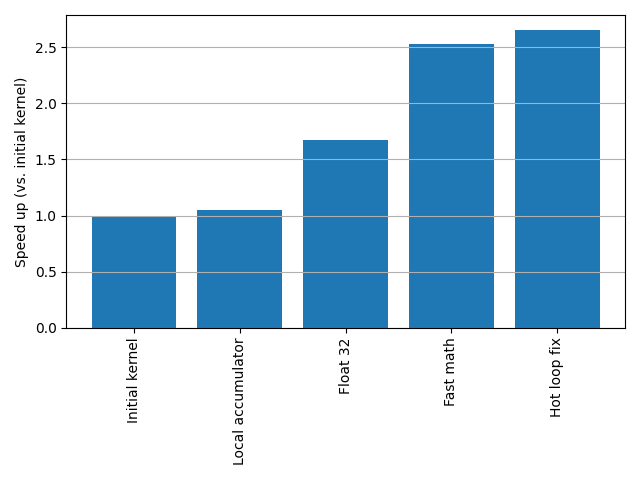
Let me remind you to always optimise with a concrete goal in mind. If this performance improvement is already enough to make your computation tractable, then I would advise stopping and counting that as a win. Otherwise, steel yourself for what comes next!
Optimisation 5: Minimise reading from global memory
We’ve previously used a local accumulation variable to minimise writes to global memory. In this section, however, we’re going to use shared memory to minimise reads from global memory.
Our problem is that each kernel needs to read through the
entirety of each of the us, vs,
ws and vis arrays. There’s a lot of
redundancy here: since each thread is fully independent, they are each
reading the same data, from start to end. But what if we could somehow
share the burden of these global memory reads amongst the threads?
A standard pattern in kernel design is for each thread in a thread block to cooperate by using shared memory as an intermediate cache. Remember that shared memory is much faster than global memory, and is visible from each thread within a thread block. In doing so, global reads reduce by a factor equal to threads per block. For a thread block with 256 threads, this will reduce global memory reads by a factor of 256.
Suppose there are 256 threads per block. Then the pattern proceeds as follows:
- The thread block allocates a shared memory array with size 256. Each thread can read and write to this array, and can see the writes of each sibling thread within the thread block.
- The thread block reads in the first 256 index values of the global memory, with each thread reading a single, unique value based on its thread ID. For example, thread 45 within the thread block reads the 45th value of the global array.
- Each thread caches its retrieved datum into a unique location in shared memory, using its thread ID as the array index. For example, thread 45 writes to the 45th index of the shared array.
- Finally, the threads cycle through each value in shared memory and performs its associated computation.
The cycle is then repeated: the next 256 values from global memory are written into shared memory, and so on, until the global memory is exhausted.
This pattern is illustrated in the following animation. This animation depicts the pattern using a thread block size of 8, which in turn means the shared memory cache is sized to 8 elements:
In pseudo-code:
PYTHON
# Create shared memory array
xs_shared = cuda.shared.array(256, dtype=np.float32)

tid = cuda.threadIdx.x  # threadId _within_ the thread block
N = len(xs_global)

# Step through the array in blocks of 256
for offset in range(0, N, 256):
    # Write all 256 values from global memory into
    if offset + tid < N:
        # Each thread in the thread block is responsible for reading a unique global memory address
        # and writing to a unique shared memory address based on its thread ID.
        xs_shared[tid] = xs_global[offset + tid]
    else:
        # Unless N is a multiple of 256, you will need to handle the remainder
        xs_shared[tid] = 0

    # Ensure the cache is fully populated before any individual thread tries to read from it
    cuda.syncthreads()

    for x in xs_shared:
        # Compute...
        pass

    # Wait for each thread to finish computation before the cache is repopulated
    cuda.syncthreads()
Some important comments:
We create shared memory by calling
cuda.shared.array(...)in each thread. But this syntax is deceptive: it looks like each thread creates its own shared array, but this allocation is actually performed just once at the thread block level. Each thread shares the same shared memory array.The
cuda.threadIdx.xis the thread ID within the thread block, ranging in this case from 0 to 255. This is not the global thread ID which we get fromcuda.grid(1).The thread ID guarantees that each thread reads from, and writes to, a unique address in global and shared memory.
Since threads within a thread block are not guaranteed to operate in lockstep (only at the warp level is this true), we need to call the synchronisation function
cuda.syncthreads(). This function acts a gate that stops threads within a given thread block from progressing until all threads have reached this point. This guarantees two things: that the cache is fully populated before we attempt to read from it; and later, that the cache is not updated until all threads have completed reading from it.-
We have to handle the case where
Nis not a multiple of 256. In the example above, on the final batch we pad the shared array with zeros on the assumption that zero is idempotent under our kernel. Other options for handling this remainder exist, such as:for i in range(min(256, N - offset)): x = xs_shared[i] # Compute...Although computing this range dynamically on every loop is usually more computationally costly.
Warning
cuda.syncthreads() acts as a gate that stops threads
from progressing until all threads within a thread block have reached
that point. But beware: cuda.syncthreads() should not be
put inside a conditional branch. A conditional branch may result in some
threads never reaching the synchronisation point and the result of doing
so is undefined and may lead to deadlock. Similarly, this advice applies
to threads that conditionally return early and therefore bypass future
synchronisation points.
Coalesced memory reads
The GPU memory system performs best when a thread block coordinates to read from a contiguous region of memory. In particular, if each thread in a thread block reads the next entry in an array, the GPU can turn all these little reads into a single, unified read instruction. For example, instead of asking the memory system to get me index 0, and then get me index 1, … and then finally index 1024, the memory system can unify these into a single instruction asking for indices 0-1024. When this happens, it is called memory coalescing.
On the other hand, if each thread reads from somewhere seemingly random, is non-sequential, or if each thread’s memory read is strided (i.e. there are gaps between each read), then the GPU can’t combine these into a single, unified read instruction. Those hundreds of reads will be queued and processed one by one. Obviously, this is not good for memory performance.
In the above example, we read from memory using the indexing
offset + tid which guarantees memory
coalescing.
Bank conflicts
Accessing shared memory comes with its own complications, one of which are bank conflicts. Shared memory operations must go via a limited number of memory banks, and if multiple threads make requests to the same memory bank the resulting conflict will force the operations to be serialised. That is, to be performed one after the other.
Modern NVIDIA GPUs have 32 memory banks. Each bank is responsible for a 32 bit chunk of memory, with bank 1 responsible for the first 32 bits, bank 2 responsible for the next 32 bits, and so on, looping around every 32 chunks. To avoid conflicts, the optimal pattern to access shared memory is to ensure that each thread within the warp reads from a unique address, modulo 32 bits.
You might notice that the 32 bit bank width seems to make bank conflicts inevitable when using 64 bit data. Some texts recommend splitting your 64 bit type into two 32 bit floats and assembling the result over two requests, although this kind of bit fiddling gets messy fast. In my experience, it is usually equally performant to use an access pattern that limits you to just two conflicting requests per bank.
Finally: there’s a special exception. If every thread accesses the same shared memory address, no conflict occurs and the value will instead be broadcast across the warp. (And this is precisely what the example code above does in its hot loop.)
Challenge
Modify the kernel to minimise global memory reads by caching the
global values from us, vs, ws,
and vis.
Start by creating shared memory arrays at the top of the kernel:
PYTHON
NTHREADS = 256
uvw_cache = cuda.shared.array((NTHREADS, 3), dtype=np.float32)
vis_cache = cuda.shared.array(NTHREADS, dtype=np.complex64)
Then proceed to complete the remaining TODOs.
Beware: We must ensure that each thread in a thread
block participates in cache generation. For example, the condition
if lmpx < img.size must no longer result in some threads
prematurely terminating. Instead, these “remainder” threads must still
continue to play their role in populating and refreshing their
associated index in the caches (to be used by the other threads in its
thread block) even though they ultimately do not write out to global
memory.
PYTHON
@cuda.jit
def kernel(us, vs, ws, vis, ls, ms, ndashes, img):
    # TODO:
    # Add the shared memory caches here

    lmpx = cuda.grid(1)

    # TODO:
    # 1. Initialize l, m, ndash
    # 2. Conditionally set l, m, ndash if lmpx < img.size
    # 3. Don't return early!

    # Initialise pixel accumulator variable
    pixel = np.complex64(0)

    # Extract input data in batches of NTHREADS items
    N = vis.size
    for offset in range(0, N, NTHREADS):
        # TODO:
        # 1. Fetch data and populate the caches
        # 2. Handle the remainder by setting cache entries to 0.

        # Wait for cache to be populated
        cuda.syncthreads()

        # Iterate over cache
        for j in range(NTHREADS):
            phase = (
                uvw_cache[j, 0] * l +
                uvw_cache[j, 1] * m +
                uvw_cache[j, 2] * ndash
            )
            sin, cos = cuda.libdevice.fast_sincosf(phase)
            pixel += vis_cache[j] * complex(cos, sin)

        # Don't start updating cache until all threads are done
        cuda.syncthreads()

    if lmpx < img.size:
img[lpx, mpx] = pixelPYTHON
@cuda.jit
def kernel(us, vs, ws, vis, ls, ms, ndashes, img):
    NTHREADS = 256
    uvw_cache = cuda.shared.array((NTHREADS, 3), dtype=np.float32)
    vis_cache = cuda.shared.array(NTHREADS, dtype=np.complex64)

    lmpx = cuda.grid(1)

    l, m, ndash = np.float32(0), np.float32(0), np.float32(0)
    if lmpx < img.size:
        lpx, mpx = divmod(lmpx, ls.shape[1])

        # Retrieve l, m and ndash coordinates associated with this pixel
        l = 2 * np.float32(np.pi) * ls[lpx, mpx]
        m = 2 * np.float32(np.pi) * ms[lpx, mpx]
        ndash = 2 * np.float32(np.pi) * ndashes[lpx, mpx]

    # Perform sum over all of the visibility data for just one pixel
    pixel = np.complex64(0)

    # Extract input data in batches of NTHREADS items
    N = vis.size
    for offset in range(0, N, NTHREADS):
        # Fetch data and populate cache
        i = offset + cuda.threadIdx.x
        if i < N:
            uvw_cache[cuda.threadIdx.x] = us[i], vs[i], ws[i]
            vis_cache[cuda.threadIdx.x] = vis[i]
        else:
            uvw_cache[cuda.threadIdx.x] = 0, 0, 0
            vis_cache[cuda.threadIdx.x] = 0

        # Wait for cache to be populated
        cuda.syncthreads()

        # Iterate over cache
        for j in range(NTHREADS):
            phase = (
                uvw_cache[j, 0] * l +
                uvw_cache[j, 1] * m +
                uvw_cache[j, 2] * ndash
            )
            sin, cos = cuda.libdevice.fast_sincosf(phase)
            pixel += vis_cache[j] * complex(cos, sin)

        # Don't start updating cache until all threads are done
        cuda.syncthreads()

    if lmpx < img.size:
        img[lpx, mpx] = pixel
Optimisation 6: Thread coarsening
Sometimes too much of a good thing can be a bad thing. When it comes to GPU threads, we want enough threads that all SMs have a number of thread blocks queued at any one time. This ensures all CUDA cores are doing work at any one time, and when a thread block needs to pause to wait for something (e.g. to access global memory) there is another thread block reading and waiting to advance its own work.
But only up to a point. Kernels have start up and initialisation costs. And in some kernels, there may be work that is repeated by every kernel that might actually be better if it were shared.
Thread coarsening is the process whereby we “dial back” the degree of parallelisation, and instead increase the computational intensity of each kernel.
Consider the following two version of the DFT kernel:
PYTHON
@cuda.jit
def dft(xs, Xs):
    k = cuda.grid(1)
    N = len(xs)

    if k < N:
        Xs_k = np.complex64(0)
        for n in range(N):
            phase = -2 * np.float32(np.pi) * k * n / N
            sin, cos = cuda.libdevice.fast_sincosf(phase)
            Xs_k += xs[n] * complex(cos, sin)

        Xs[k] = Xs_k

@cuda.jit
def dft_coarsened(xs, Xs):
    THREAD_COARSEN = 4
    N = len(xs)

    # Allocate local arrays to store:
    # 1. The k index
    # 2. The respective accumulator variable
    ks = cuda.local.array(THREAD_COARSEN, dtype=np.int64)
    Xs_ks = cuda.local.array(THREAD_COARSEN, dtype=np.complex64)

    # Initialise the local arrays
    for i in range(THREAD_COARSEN):
        ks[i] = cuda.grid(1) + i * cuda.gridsize(1)
        Xs_ks[i] = 0  # zero each element of the array

    for n in range(N):
        # Prefetch global memory item
        x = xs[n]
        # Precompute part of the phase term
        partial_phase = -2 * np.float32(np.pi) * n / N

        for i in range(THREAD_COARSEN):
            phase = ks[i] * partial_phase
            sin, cos = cuda.libdevice.fast_sincosf(phase)
            Xs_ks[i] += x * complex(cos, sin)

    for i in range(THREAD_COARSEN):
        k = ks[i]
        if k < N:
            Xs[k] = Xs_ks[i]
In the original DFT kernel, each thread is responsible for computing
just the k’th index of Xs. Compare this to the
coarsened version, where each thread computes four distinct indices of
Xs: k, k + gridsize,
…k + 3 * gridsize.
How does it do this?
- We set the thread coarsening factor,
THREAD_COARSEN, as a constant value within the kernel. - We create two locally-allocated arrays, one for the k values and one for accumulator variables.
- On each iteration of
n, we compute for the partial sum of each of the k values. - By doing so, we amortise the cost of accessing
xs[n]and computing (part of) the phase value across the four indices.
In fact, if you do your own experimentation with this code, you’ll see that almost all of the performance win is due to pre-computing the partial phase term.
Advanced note: we define THREAD_COARSEN
as a constant within the kernel. You might be tempted to pass
this as an argument so that you can modify the thread coarsening factor
dynamically. Unfortunately, the kernel requires that local arrays are
sized statically, which means that their size is known at compile time.
If it were sized by a function parameter, then this array size would
only be known at the time the function is called, that is, at
runtime. This actually has some flow-on benefits for us: since
the compiler knows the size of THREAD_COARSEN at compile
time, it also knows the size of the loops over
THREAD_COARSEN, and at its discretion it may choose to unroll these
loops for performance gains.
Challenge
On your machine, experiment with benchmarking different thread
coarsening factors for the dft_coarsened kernel. What is
the ideal factor?
PYTHON
N = 500_000
xs = cupy.random.normal(size=N, dtype=np.float32) + 1j * cupy.random.normal(size=N, dtype=np.float32)
Xs = cupy.zeros_like(xs)

# Set THREAD_COARSEN both here and in the kernel definition. Try values for 1, 2, 3, 4, 6, 8
threads = 128
nblocks = math.ceil(N / threads / THREAD_COARSEN)
print(cupyx.profiler.benchmark(lambda: dft_coarsened[nblocks, threads](xs, Xs), n_repeat=1, n_warmup=1))On my own machine, I saw best performance when
THREAD_COARSEN was set to 4, but it will vary based on the
kernel, the GPU, and the problem size. Even larger thread coarsening
factors risk a number of problems:
- The number of thread blocks may decrease to the point where the GPU’s SMs are not well utilised.
- The memory requirements of each thread will obstruct the number of simultaneous thread blocks that can be scheduled on a single SM.
- Eventually, the memory required for a single thread may become so large that the local register storage “spills” out into global memory. When this happens, some of our local variables end up being actually stored in global memory, which is disastrous for performance.
Challenge
Modify the imaging kernel to use a thread coarsening factor of 3.
Start by creating some local arrays:
PYTHON
THREAD_COARSEN = 3
lmns = cuda.local.array((THREAD_COARSEN, 3), np.float32)
pixels = cuda.local.array(THREAD_COARSEN, np.complex64)
And then complete the remainder of the TODOs:
PYTHON
@cuda.jit
def kernel(us, vs, ws, vis, ls, ms, ndashes, img):
    NTHREADS = 256
    uvw_cache = cuda.shared.array((NTHREADS, 3), dtype=np.float32)
    vis_cache = cuda.shared.array(NTHREADS, dtype=np.complex64)

    # TODO:
    # Allocate the local arrays here

    for i in range(THREAD_COARSEN):
        lmpx = cuda.grid(1) + i * cuda.gridsize(1)
        if lmpx < img.size:
            # TODO:
            # Initialise the values of both of the static arrays

    # Extract input data in batches of NTHREADS items
    N = vis.size
    for offset in range(0, N, NTHREADS):
        # Fetch data and populate cache
        i = offset + cuda.threadIdx.x
        if i < N:
            uvw_cache[cuda.threadIdx.x] = us[i], vs[i], ws[i]
            vis_cache[cuda.threadIdx.x] = vis[i]
        else:
            uvw_cache[cuda.threadIdx.x] = 0, 0, 0
            vis_cache[cuda.threadIdx.x] = 0

        # Wait for cache to be populated
        cuda.syncthreads()

        # Iterate over cache
        for j in range(NTHREADS):
            for i in range(THREAD_COARSEN):
                phase = (
                    # TODO:
                    # Compute phase using local arrays
                )
                sin, cos = cuda.libdevice.fast_sincosf(phase)
                pixels[i] += vis_cache[j] * complex(cos, sin)

        # Don't start updating cache until all threads are done
        cuda.syncthreads()

    for i in range(THREAD_COARSEN):
        lmpx = cuda.grid(1) + i * cuda.gridsize(1)
        # TODO:
# Write out each of the accumulated pixel values to global memoryPYTHON
@cuda.jit
def kernel(us, vs, ws, vis, ls, ms, ndashes, img):
    NTHREADS = 256
    uvw_cache = cuda.shared.array((NTHREADS, 3), dtype=np.float32)
    vis_cache = cuda.shared.array(NTHREADS, dtype=np.complex64)

    THREAD_COARSEN = 3
    lmns = cuda.local.array((THREAD_COARSEN, 3), np.float32)
    pixels = cuda.local.array(THREAD_COARSEN, np.complex64)

    for i in range(THREAD_COARSEN):
        lmpx = cuda.grid(1) + i * cuda.gridsize(1)
        if lmpx < img.size:
            lpx, mpx = divmod(lmpx, ls.shape[1])

            # Retrieve l, m and ndash coordinates associated with this pixel
            lmns[i, 0] = 2 * np.float32(np.pi) * ls[lpx, mpx]
            lmns[i, 1] = 2 * np.float32(np.pi) * ms[lpx, mpx]
            lmns[i, 2] = 2 * np.float32(np.pi) * ndashes[lpx, mpx]

            # Perform sum over all of the visibility data for just one pixel
            pixels[i] = np.complex64(0)

    # Extract input data in batches of NTHREADS items
    N = vis.size
    for offset in range(0, N, NTHREADS):
        # Fetch data and populate cache
        i = offset + cuda.threadIdx.x
        if i < N:
            uvw_cache[cuda.threadIdx.x] = us[i], vs[i], ws[i]
            vis_cache[cuda.threadIdx.x] = vis[i]
        else:
            uvw_cache[cuda.threadIdx.x] = 0, 0, 0
            vis_cache[cuda.threadIdx.x] = 0

        # Wait for cache to be populated
        cuda.syncthreads()

        # Iterate over cache
        for j in range(NTHREADS):
            for i in range(THREAD_COARSEN):
                phase = (
                    uvw_cache[j, 0] * lmns[i, 0] +
                    uvw_cache[j, 1] * lmns[i, 1] +
                    uvw_cache[j, 2] * lmns[i, 2]
                )
                sin, cos = cuda.libdevice.fast_sincosf(phase)
                pixels[i] += vis_cache[j] * complex(cos, sin)

        # Don't start updating cache until all threads are done
        cuda.syncthreads()

    for i in range(THREAD_COARSEN):
        lmpx = cuda.grid(1) + i * cuda.gridsize(1)
        if lmpx < img.size:
            lpx, mpx = divmod(lmpx, ls.shape[1])
            img[lpx, mpx] = pixels[i]
An aside: You might think that it might be more efficient to prefetch the \(u, v, w\) terms prior to the loop over the thread coarsening factor. That is, something like this:
PYTHON
# Iterate over cache
for j in range(NTHREADS):
    u, v, w = uvw_cache[j]
    for i in range(THREAD_COARSEN):
        phase = (
            u * lmns[i, 0] +
            v * lmns[i, 1] +
            w * lmns[i, 2]
        )
        sin, cos = cuda.libdevice.fast_sincosf(phase)
        pixels[i] += vis_cache[j] * complex(cos, sin)
This hot loop optimisation avoids unnecessary accesses to shared memory by instead placing those values into registers which are faster. However, at least for my environment, this version turned out to be actually slower (and I don’t know why!). In both versions, the compiler should recognise that these are in fact the same pattern and that it should compile to whichever method is faster, but this is clearly a case where the compiler fails us. As always, benchmark ruthlessly.
Optimisation 7: Force FMA instructions
Fused multiply add (FMA) instructions are a special hardware instruction that combines both a multiplication and addition as a single operation. In pseudo-code:
If we can rewrite paired multiply-then-add operations as single FMA operations, we can significantly improve throughput — in the best case approaching a 2x speedup for the arithmetic portion of the kernel. (In fact, the numbers for GPU floating point performance that you’ll see NVIDIA or AMD advertising assume that 100% of your code is pure FMA instructions – which almost no non-trivial kernel is capable of achieving.)
The CUDA compiler should make an effort to automatically insert FMA instructions into your code, but it has been my experience that it is less than perfect.
Let’s consider the expression from our inner loop:
How would we write this as an FMA instruction? The first and most
immediate problem we encounter here is that cuda.fma is
defined strictly for np.float32 and np.float64
types, whereas here we are dealing with complex numbers. Let’s expand
this a little into real and imaginary components:
PYTHON
pixels[i] += complex(
    datum.real * cos - datum.imag * sin,  # real component
    datum.real * sin + datum.imag * cos   # imaginary component
)
If we consider just the real component for a moment, then we can write this as two FMA instructions:
PYTHON
pixels_real[i] = cuda.fma(datum.real, cos, pixels_real[i])
pixels_real[i] = cuda.fma(datum.imag, -sin, pixels_real[i])
Check that this makes sense to you!
Challenge
We are going to rewrite
pixels[i] += vis_cache[j] * complex(cos, sin) as a sequence
of 4 FMA instructions.
There’s a small problem here. Whilst we can retrieve the real and
imaginary components of a complex number with the .real and
.imag attributes respectively, we aren’t able to modify
these values. To simplify the presentation here, we will create the
accumulation array pixel as 2D array, with the second
dimension corresponding to the real and imaginary components:
(You will need to update the code that zeroes this array too.)
Once you have done this, attempt to write out the inplace complex addition as a sequence of 4 FMA instructions. As a hint, the first looks like this:
Finally, we arrive at a kernel that looks like that shown below.
PYTHON
@cuda.jit
def kernel(us, vs, ws, vis, ls, ms, ndashes, img):
    NTHREADS = 256
    uvw_cache = cuda.shared.array((NTHREADS, 3), dtype=np.float32)
    vis_cache = cuda.shared.array(NTHREADS, dtype=np.complex64)

    THREAD_COARSEN = 3
    lmns = cuda.local.array((THREAD_COARSEN, 3), np.float32)
    pixels = cuda.local.array((THREAD_COARSEN, 2), np.float32)

    for i in range(THREAD_COARSEN):
        lmpx = cuda.grid(1) + i * cuda.gridsize(1)
        if lmpx < img.size:
            lpx, mpx = divmod(lmpx, ls.shape[1])

            # Retrieve l, m and ndash coordinates associated with this pixel
            lmns[i, 0] = 2 * np.float32(np.pi) * ls[lpx, mpx]
            lmns[i, 1] = 2 * np.float32(np.pi) * ms[lpx, mpx]
            lmns[i, 2] = 2 * np.float32(np.pi) * ndashes[lpx, mpx]

            # Perform sum over all of the visibility data for just one pixel
            pixels[i] = 0, 0

    # Extract input data in batches of NTHREADS items
    N = vis.size
    for offset in range(0, N, NTHREADS):
        # Fetch data and populate cache
        i = offset + cuda.threadIdx.x
        if i < N:
            uvw_cache[cuda.threadIdx.x] = us[i], vs[i], ws[i]
            vis_cache[cuda.threadIdx.x] = vis[i]
        else:
            uvw_cache[cuda.threadIdx.x] = 0, 0, 0
            vis_cache[cuda.threadIdx.x] = 0

        # Wait for cache to be populated
        cuda.syncthreads()

        # Iterate over cache
        for j in range(NTHREADS):
            for i in range(THREAD_COARSEN):
                phase = cuda.fma(
                    uvw_cache[j, 0],
                    lmns[i, 0],
                    cuda.fma(uvw_cache[j, 1], lmns[i, 1], uvw_cache[j, 2] * lmns[i, 2]),
                )
                sin, cos = cuda.libdevice.fast_sincosf(phase)
                pixels[i, 0] = cuda.fma(vis_cache[j].real, cos, pixels[i, 0])
                pixels[i, 0] = cuda.fma(vis_cache[j].imag, -sin, pixels[i, 0])
                pixels[i, 1] = cuda.fma(vis_cache[j].real, sin, pixels[i, 1])
                pixels[i, 1] = cuda.fma(vis_cache[j].imag, cos, pixels[i, 1])

        # Don't start updating cache until all threads are done
        cuda.syncthreads()

    for i in range(THREAD_COARSEN):
        lmpx = cuda.grid(1) + i * cuda.gridsize(1)
        if lmpx < img.size:
            lpx, mpx = divmod(lmpx, ls.shape[1])
            img[lpx, mpx] = complex(pixels[i, 0], pixels[i, 1])
You might wonder: did the compiler fail to use FMA instructions because we were using complex numbers? After all, complex numbers ‘wrap’ a 2-tuple of floats and this indirection might obscure the underlying operations. Try experimenting with this: if we retain the real and imaginary parts stored seperately as we have below, and write out the real and imaginary components separately using normal multiplication and addition operators, do you see the same speedup?
Optimisation 8: Warp shuffling (optional)
I hesitated to include this final section as it in fact doesn’t substantially improve the speed of our code, nor is it idiomatic. In fact, I would advise that the previous version of the kernel is the right place to stop and uses the most recognisable patterns.
However, I do want you to be aware of a few more intrinsics that might come in handy for your particular use case. Namely, there is a set of warp level intrinsics that let you move data directly between registers amongst members of a warp (being the set of 32 threads that execute in lockstep). Normally, these intrinsics might be used as part of a reduction operation, or they might be used to broadcast a single value to the other members of the warp. Warp communication should usually be slightly faster than communicating values via shared memory.
We’re going to use these intrinsics to replace our shared memory
cache. Instead of using shared memory, each warp member will load a
unique (and successive) value of each of \(u,
v, w\) and \(vis\). But then we
will have each thread “pass the parcel” 32 times using
cuda.shfl_sync(), effectively daisychaining the input data
amongst the warp, before they continue by reading in the next chunk of
input data.
cuda.shfl_sync() accepts 3 parameters:
- The first is a mask which indicates which of the warp threads are to
participate in the shuffle. Since we want every thread to play its part,
we set this to
0xFFFFFFFF. - The second parameter is the value to shuffle. This is the value that this thread offers up, and if another warp member targets us, this is the value they will receive.
- The third parameter is the source lane ID. Ranging from 0 to 31, this identifies the warp member whose value we want to receive.
We can use cuda.shfl_sync() to act as a warp-wide cache
as demonstrated by the following pseudo code:
PYTHON
warpid = cuda.threadIdx.x % cuda.warpsize
nextwarpid = (cuda.threadIdx.x + 1) % cuda.warpsize

N = len(xs)
for i in range(0, N, cuda.warpsize):
    x = xs[i + warpid]
    for _ in range(cuda.warpsize):
        # Do some computation with x

        # Then daisy chain x amongst the warp
        x = cuda.shfl_sync(0xFFFFFFFF, x, nextwarpid)
There’s no need to use synchronisation calls because the warp
executes in lockstep (however, be careful to avoid divergence at any
place where shfl_sync is called).
Challenge
Remove the shared memory cache from our kernel and instead implement a warp-wide cache that follows the pattern set out above.
Note that cuda.shfl_sync() is limited only to floats,
doubles. For complex values we’ll have to transmit the real and
imaginary parts separately, e.g.:
x = complex(cuda.shfl_sync(0xFFFFFFFF, nextwarpid, x.real), cuda.shfl(0xFFFFFFFF, nextwarpid, x.imag)).
Shared memory is the idiomatic way to cache data and avoid global
memory operations: it is what you will see in most CUDA tutorials, and
is most appropriate when the cache is large. For the sake of exposing
you to warp level intrinsics, however, this code demonstrates how
cuda.shfl_sync can act as a substitute cache that has equal
performance.
Note that the threadsize for this kernel can be set to any arbitrary multiple of 32. In my own benchmarking, using 512 threads had the best performance.
PYTHON
@cuda.jit
def kernel(us, vs, ws, vis, ls, ms, ndashes, img):
    THREAD_COARSEN = 3
    lmns = cuda.local.array((THREAD_COARSEN, 3), np.float32)
    pixels = cuda.local.array((THREAD_COARSEN, 2), np.float32)

    for i in range(THREAD_COARSEN):
        lmpx = cuda.grid(1) + i * cuda.gridsize(1)
        if lmpx < img.size:
            lpx, mpx = divmod(lmpx, ls.shape[1])

            # Retrieve l, m and ndash coordinates associated with this pixel
            lmns[i, 0] = 2 * np.float32(np.pi) * ls[lpx, mpx]
            lmns[i, 1] = 2 * np.float32(np.pi) * ms[lpx, mpx]
            lmns[i, 2] = 2 * np.float32(np.pi) * ndashes[lpx, mpx]

            # Perform sum over all of the visibility data for just one pixel
            pixels[i, 0] = 0
            pixels[i, 1] = 0

    WARPSIZE = cuda.warpsize
    warpid = cuda.threadIdx.x % WARPSIZE
    nextwarpid = (cuda.threadIdx.x + 1) % WARPSIZE

    # Extract input data in batches of WARPSIZE items
    N = vis.size
    for offset in range(0, N, WARPSIZE):
        # Each warp member loads its respective visibility data
        i = offset + warpid
        if i < N:
            u, v, w = us[i], vs[i], ws[i]
            datum = vis[i]
        else:
            u, v, w, = np.float32(0), np.float32(0), np.float32(0)
            datum = np.complex64(0)

        # Iterate over warp cache
        for _ in range(WARPSIZE):
            for i in range(THREAD_COARSEN):
                phase = cuda.fma(
                    u,
                    lmns[i, 0],
                    cuda.fma(v, lmns[i, 1], w * lmns[i, 2]),
                )
                sin, cos = cuda.libdevice.fast_sincosf(phase)
                pixels[i, 0] = cuda.fma(datum.real, cos, pixels[i, 0])
                pixels[i, 0] = cuda.fma(datum.imag, -sin, pixels[i, 0])
                pixels[i, 1] = cuda.fma(datum.real, sin, pixels[i, 1])
                pixels[i, 1] = cuda.fma(datum.imag, cos, pixels[i, 1])

            # Daisychain the values around members of the warp
            u = cuda.shfl_sync(0xFFFFFFFF, u, nextwarpid)
            v = cuda.shfl_sync(0xFFFFFFFF, v, nextwarpid)
            w = cuda.shfl_sync(0xFFFFFFFF, w, nextwarpid)

            datum = complex(
                cuda.shfl_sync(0xFFFFFFFF, datum.real, nextwarpid),
                cuda.shfl_sync(0xFFFFFFFF, datum.imag, nextwarpid)
            )

    for i in range(THREAD_COARSEN):
        lmpx = cuda.grid(1) + i * cuda.gridsize(1)
        if lmpx < img.size:
            lpx, mpx = divmod(lmpx, ls.shape[1])
            img[lpx, mpx] = complex(pixels[i, 0], pixels[i, 1])
Final comparison
We have made substantial performance gains, at just over 13 times the performance of the initial kernel: