How to Automate the Boring Bits

Overview

Teaching: 45 min
Exercises: 45 min

Questions

How can automation improve my current workflow?

How can I automate my current work?

How can I ensure that my workflow is reproducible on different computers?

What workflow management tools are available?

Objectives

Learn to streamline the routine tasks in your research - from downloading remote data to managing reproducible computational environments - so you can focus on discovery.

Overview

Why automate?

Automation helps streamline repetitive tasks, reduce errors, and save time, allowing you to focus on analysis and discovery. By incorporating automation techniques into your research workflows, you can improve the efficiency, consistency, and reproducibility of your work, ultimately leading to more reliable and impactful scientific discoveries.

Common repetitive tasks in research:

Research often involves a variety of repetitive tasks that can benefit from automation, including:

Data retrieval: Regularly downloading large datasets from remote servers or online repositories.
Data preprocessing: Cleaning, filtering, and formatting raw data to prepare it for analysis.
Data analysis: Running the same analysis scripts on multiple datasets or subsets of data.
Report generation: Creating standardized reports or visualizations from analysis results.
Environment setup: Configuring computational environments with specific software dependencies for different projects.

How automation can help:

Efficiency: Automating repetitive tasks can save significant time and effort, allowing you to focus on more complex and creative aspects of your work.
Consistency: Automated workflows ensure that tasks are performed the same way every time, reducing the risk of human error and increasing the reliability of results.
Reproducibility: By automating the setup of computational environments and the execution of analysis scripts, you can easily reproduce your work and share it with others.
Scalability: Automation makes it easier to scale up analyses to larger datasets or more complex workflows without a proportional increase in manual effort.
Documentation: Automated workflows often include built-in documentation and logging, making it easier to track what was done and troubleshoot any issues that arise.

Tools and techniques for automation:

Scripting languages: Use languages like Python or Bash to write scripts that automate repetitive tasks.
Workflow management tools: Tools like Make and Nextflow can help manage complex workflows with multiple dependencies and parallel tasks.
Version control: Use Git to track changes to scripts and workflows, ensuring that you can revert to previous versions if needed.
Continuous integration: Set up continuous integration (CI) pipelines to automatically run tests and analyses whenever changes are made to your code or data.

Leveraging Large Language Models (LLMs) for Automation:

Large Language Models (LLMs) like ChatGPT and (GitHub) CoPilot can assist in automating various aspects of research by providing intelligent suggestions, generating code snippets, and even automating documentation tasks. As a bonus, many of these are free for academic use, or are included as part of your organisations enterprise software agreements. Here are some ways LLMs can be utilized:

Code Generation: LLMs can generate code snippets for common tasks, reducing the time spent writing boilerplate code.
Data Analysis: LLMs can assist in writing complex data analysis scripts by providing suggestions and examples.
Documentation: Automatically generate documentation for code, workflows, and research findings, ensuring consistency and saving time.
Testing: LLMs can suggest tests for your code, reducing the time writing boilerplate code.

Verify LLM outputs

A very important note about the use of LLMs (or any assistive tools) is that their output is not guaranteed to be: error free, up-to-date, appropriate, or logically sound. You are ultimately responsible for your research and software and so you should carefully validate the information that you get from these tools. Think of these tools as an untrusted colleague or random stack-overflow contributor with low reputation - you need to think critically about what is being presented to you.

Today’s focus

In this workshop we are going to start with a commonly disliked, overlooked, and time consuming aspect of research - data cleaning - and learn some techniques to automate the process. The scenario that are going to work on is one that I had to struggle with during my PhD - preparing catalogues of radio sources for analysis. At the time, tools such as AstroPy were just being developed, and were certainly not as widely used as today. Not only that, but the data that I was using wasn’t avaialble in consistent formats - different research groups provided data via different online services which had very different data formats. Today the world is a little nicer, as many people have realised the benefits of FAIR data not only to people who want to use the data, but also those who want to be recognised for publishing it.

The task that we will focus on today is the following:

Obtain a catalogue of data data for a given radio survey
Clean and filter the data
Convert the data into a standard format

We will firstly look at how we would do all of this manually (because thats how you do everything the first time), and then learn some tools that will help us to automate the process.

A workflow for humans

Download the AT20G dataset from this repo (a subset of the entire catalogue from ViZieR)
Separate the meta data from the table data (starts with #)
Remove the second two lines of the table header (units and ----)
Count the number of rows in the data, record for later use
Correct the data types of the columns (currently most are strings, thanks to missing data)
Remove all rows with no 5/8GHz measurements (columns S8 and S5)
Keep only rows with 12 <= RA <= 18 (hours)
Count the number of rows rejected/remaining, record for later use
Delete all columns from Ep -> Sp
Save the filtered file for analysis work as AT20G_clean.csv

What tools can we use?

Excel or similar is a good enough tool, widely available, that you can use to inspect and edit your data.

If a new version of that catalogue comes out (same format, adjusted values or more rows), how long does it take to redo this?

If you need to add extra filtering steps, how much work do you need to redo?

When you write up your methods section and need to describe this filtering process, where have you recorded it? How do you know how many rows passed each criteria?

You want to change your analysis so that you can see the distribution of sources on sky before/after the filtering is done. Do you have a dataset that would allow this?

Let’s now take our workflow and make it a workflow for computers.

A workflow for computers

For each of the steps above we need to identify a tool.

Overall we have three main things we are doing with our data:

Downloading data
Separating lines of a file based on content
Filtering rows / columns of a table

While there are many different options available, and we could potentially use one tool to do everything, I find it a lot easier to choose the right tool for the right job. This can mean you need to learn a few different tools, but you don’t need to become expert in each tool.

The tools that we are going to use today are:

wget or curl for downloading files
grep for selecting lines of a file based on content
python3/pandas for manipulating our table

Downloading data from remote sources

wget and curl are two programs that are usually available on most systems. They both perform the same task - connect to a url and saves the content to a file. If you hit a url which is a website, you’ll end up with a .html file. If you connect to a file then you’ll get the file itself.

Download our AT20g.tsv file using either of the following options (depending on what is available on your system).

# Download a single file
wget https://raw.githubusercontent.com/ADACS-Australia/2025-ASA-ECR-WorkshopSeries/refs/heads/gh-pages/data/Workshop1/AT20G.tsv

You should see some output like this, and the AT20G.tsv file in your current directory.

--2025-04-17 11:49:35--  https://raw.githubusercontent.com/ADACS-Australia/2025-ASA-ECR-WorkshopSeries/refs/heads/gh-pages/data/Workshop1/AT20G.tsv
Resolving raw.githubusercontent.com (raw.githubusercontent.com)... 185.199.110.133, 185.199.109.133, 185.199.108.133, ...
Connecting to raw.githubusercontent.com (raw.githubusercontent.com)|185.199.110.133|:443... connected.
HTTP request sent, awaiting response... 200 OK
Length: 550370 (537K) [text/plain]
Saving to: ‘AT20G.tsv’

AT20G.tsv           100%[===================>] 537.47K  --.-KB/s    in 0.005s  

2025-04-17 11:49:36 (106 MB/s) - ‘AT20G.tsv’ saved [550370/550370]

And if we are using curl, the syntax is almost the same:

# Download a single file
curl -O https://raw.githubusercontent.com/ADACS-Australia/2025-ASA-ECR-WorkshopSeries/refs/heads/gh-pages/data/Workshop1/AT20G.tsv

  % Total    % Received % Xferd  Average Speed   Time    Time     Time  Current
                                 Dload  Upload   Total   Spent    Left  Speed
100  537k  100  537k    0     0  20.5M      0 --:--:-- --:--:-- --:--:-- 20.1M

Again the file will end up in the current directory.

Now that we have figured out how to download the file automatically, we should copy the commands that we used for reference later on.

Make a workflow file

Make a file called workflow.txt which we’ll use to create our automated workflow. Add the wget/curl command that you used above into this file.

Separating data from meta-data

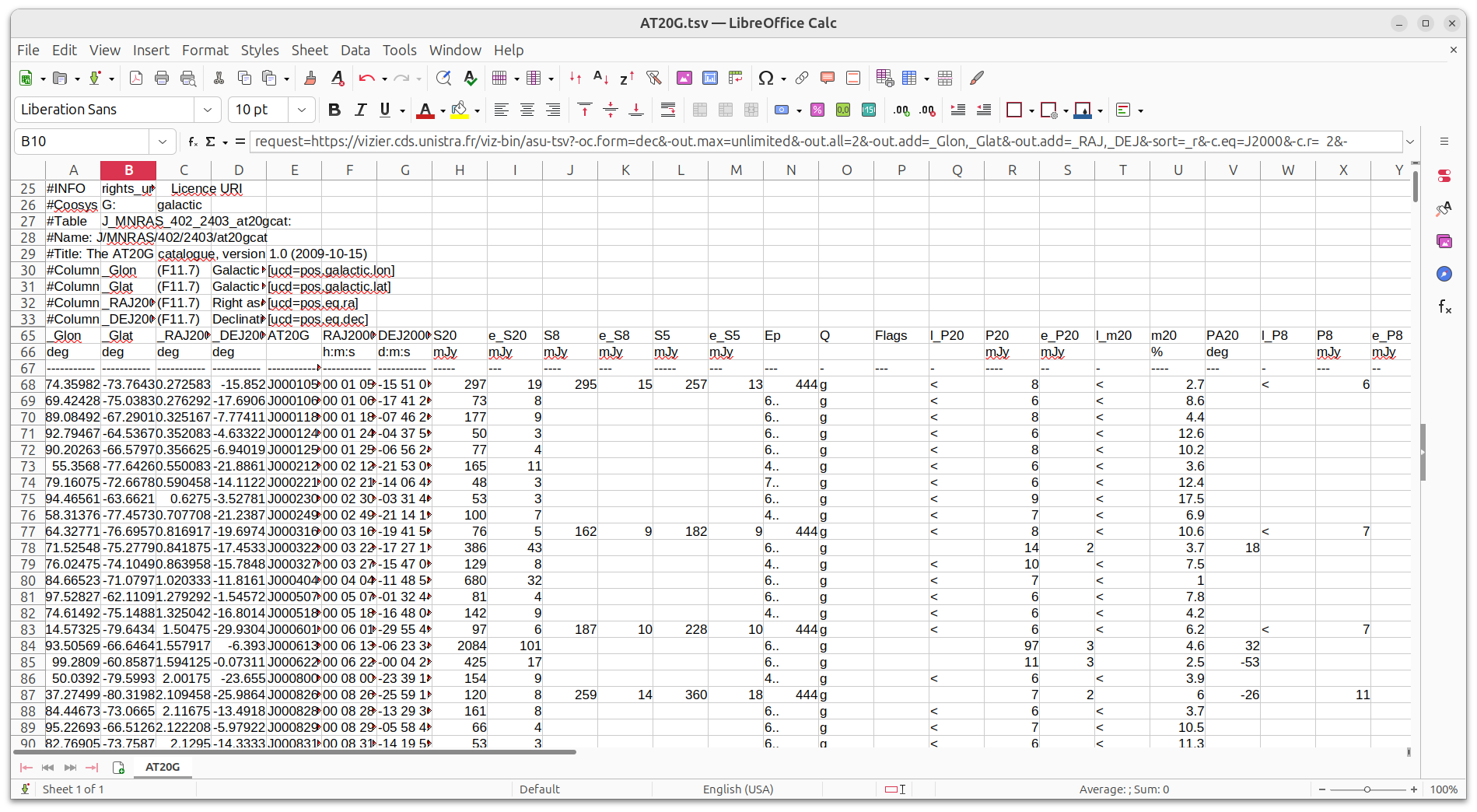
We should now have a file called AT20G.tsv in our working directory, which looks like the following:

AT20G.tsv

#
#   VizieR Astronomical Server vizier.cds.unistra.fr
#    Date: 2025-04-10T06:17:11 [V7.4.6]
#   In case of problem, please report to:       cds-question@unistra.fr
#
#
#Coosys J2000:  eq_FK5 J2000
#INFO   service_protocol=ASU      IVOID of the protocol through which the data was retrieved
#INFO   request_date=2025-04-10T06:17:11          Query execution date
#INFO   request=https://vizier.cds.unistra.fr/viz-bin/asu-tsv?-oc.form=dec&-out.max=unlimited&-out.all=2&-out.add=_Glon,_Glat&-out.add=_RAJ,_DEJ&-sort=_r&-c.eq=J2000&-c.r=  2&-c.u=arcmin&-c.geom=r&-source=J/MNRAS/402/> 2403/at20gcat&-order=I&-out=AT20G&-out=RAJ2000&-out=DEJ2000&DEJ2000=&gt;-30 & &lt;0&-out=S20&-out=e_S20&-out=S8&-out=e_S8&-out=S5&-out=e_S5&-out=Ep&-out.all=2&-out=Q&-out=Flags&-out=l_P20&-out=P20&-out=e_P20&-out=l_m20&-out=m20&-out=PA20&-out=l_P8&-out=P8&-out=e_P8&-out=l_m8&-out=m8&-out=PA8&-out=l_P5&-out=P5&-out=e_P5&-out=l_m5&-out=m5&-out=PA5&-out=Sp&Sp=Sp&-out.all=2&       Full request URL (POST)
...
#Column PA5     (I3)    [-90/90]? Position angle at 5GHz        [ucd=pos.posAng]
#Column Sp      (A2)    SPECFIND of radio surveys with this source (Vollmer et al., Cat. VIII/85)       [ucd=meta.ref.url]
_Glon   _Glat   _RAJ2000        _DEJ2000        AT20G   RAJ2000 DEJ2000 S20     e_S20   S8      e_S8    S5      e_S5    Ep      Q       Flags   l_P20   P20     e_P20   l_m20   m20     PA20    l
_P8     P8      e_P8    l_m8    m8      PA8     l_P5    P5      e_P5    l_m5    m5      PA5     Sp
deg     deg     deg     deg             "h:m:s" "d:m:s" mJy     mJy     mJy     mJy     mJy     mJy                                     mJy     mJy             %       deg             mJy     m
Jy              %       deg             mJy     mJy             %       deg
-----------     -----------     -----------     -----------     --------------  -----------     -----------     -----   ---     ----    ---     -----   ---     ---     -       ---     -       -
---     --      -       ----    ---     -       ---     --      -       -----   ---     -       ----    -       -       -----   ---     --
074.3598240     -73.7643280     000.2725833     -15.8520000     J000105-155107  00 01 05.42     -15 51 07.2       297    19      295     15       257    13     444     g               <          8             <        2.7            <         6             <         2.0           <          6            <         2.3           Sp
069.4242750     -75.0383103     000.2762917     -17.6906111     J000106-174126  00 01 06.31     -17 41 26.2        73     8                                     6..     g               <        
...
093.5244966     -61.6186061     359.3548750      -1.8704444     J235725-015213  23 57 25.17     -01 52 13.6       124     6                                     6..     p               <         10             <        8.0                                                                                                            Sp
081.4390180     -69.8275875     359.3803750     -11.4274444     J235731-112538  23 57 31.29     -11 25 38.8       804    38                                     6..     p                         12      2               1.5    -86                                                                                                     Sp
087.0646275     -67.0857923     359.5407500      -8.0010278     J235809-080003  23 58 09.78     -08 00 03.7        67     3                                     6..     p               <          6             <        9.0                                                                                                            Sp
083.6389933     -69.0391655     359.5458333     -10.3355556     J235811-102008  23 58 11.00     -10 20 08.0      1243    59                                     6..     p               <         12             <        1.0                                                                                                            Sp
021.2857573     -78.1419382     359.5700417     -28.8926944     J235816-285333  23 58 16.81     -28 53 33.7       147    10      219     12       178     9     444     p               <          6             <        4.3            <         9             <         4.1           <          6            <         3.4           Sp
058.1557506     -76.5292565     359.8314583     -20.7988333     J235919-204755  23 59 19.55     -20 47 55.8       100     4      222      7       257     8     444     p       e       <          7             <       10.4            <        13             <        12.9           <          7            <         4.7           Sp
089.5191701     -66.1071830     359.8830000      -6.6621944     J235931-063943  23 59 31.92     -06 39 43.9       113     6                                     6..     g               <          8             <        7.2                                                                                                            Sp
095.7351629     -60.6265524     359.9041667      -0.5206389     J235937-003114  23 59 37.00     -00 31 14.3       272    14                                     7..     g                          6      1               2.3      0                                                                                                     Sp

The structure of the file is as follows:

a lot of metadata (rows starting with #)
header information for the table columns (three rows)
data for the table with tabs separating each entry

In order to separate the metadata rows we’ll use a program called grep which is great for selecting/deselecting lines of a file based on a string pattern match.

Select all the lines that start with a #
grep -e '^#' AT20G.tsv
Here we are telling grep to print out all the rows of the given file that have a # as the first character on the line (^ represents the start of the line). Type this into your terminal and review the output.

Save the header to a separate file

We can direct the output of grep into a file using the redirection operator >. For example:
grep -e '^#' > AT20G_header.txt
Do this now and check that the new file exists and has all the meta data in it.

If we want to make another file which has the meta-data stripped from it, we can instruct grep to return all non matchin rows using the -v operator.

grep -v -e '^#' AT20G.tsv

We could pipe these results to an intermediate file for further processing, however grep allows us to chain many patterns together. Thus we can have a single command like the following for our filtering:

grep -v -e '^#' -e '^-' -e '^deg' -e '^$' AT20G.tsv

Where we use the following:

-v show NON matching rows
-e add expression for matching
^# match lines starting with # (the metadata)
^deg lines starting with deg (the second line in the header)
^- match lines starting with - (the thrid line in the header)
^$ empty lines (^ and $ represent the first/last char in a line, so ^$ is a shortcut for empty lines)

Note: the ordering of the match patterns doesn’t affect the content of the output.

Use less to page output

The previous grep command will produce pages of output, and the key results that we are looking for are on the first page only. We can page the output by piping the results to a program called less:
<command> | less
(press Q to close the program)

I recommend you do this with the above grep command to see that the header is correct.

Update your workflow file

Use the grep functions that we worked with above, to add two new lines to your workflow file:

Save the meta-data to a file called AT02G_header.txt

Save the table data to a file called AT20G_table.tsv

my workflow file

# Download the data
wget https://raw.githubusercontent.com/ADACS-Australia/2025-ASA-ECR-WorkshopSeries/refs/heads/gh-pages/data/Workshop1/AT20G.tsv
# Save the meta-data
grep -e '^#' AT20G.tsv > AT20G_header.txt
# Save just the table with a 1 line header
grep -v -e '^#' -e '^-' -e '^deg' -e '^$' AT20G.tsv > AT20G_table.tsv

Note that I’ve added some comments (starting with #) to this file so that I can recall what the different commands are supposed to be doing.

Cleaning the table data

The command line tools we used so far are great for simple options, but tring to filter a table based on string matching is a very hard task. Therefore we will reach into our toolbox for another tool, this time the pandas module in python.

For this next section to work you’ll need to have python3 installed with both the pandas and numpy modules. numpy is a dependency for pandas so you can just install pandas and you’ll have everything you need.

To check if you have pandas installed you can run the following:

python3 -c 'import pandas'

If you get no output then everything is fine, if you get an error message then you’ll need to have pandas installed using pip install pandas or conda install pandas, depending on how your python environment is set up.

We’ll work from the command line for now so lets open up python and import the modules that we’ll be using:

import pandas as pd
import numpy as np

load our table with `pandas`

Use the pd.read_csv function to load the table and then view a summary of the table. pandas refers to tables as a “data frame” so df is the most commonly used as the name for this variable.

df = pd.read_csv('AT20G_table.tsv', delimiter='\t')
df

          _Glon      _Glat    _RAJ2000   _DEJ2000           AT20G      RAJ2000      DEJ2000    S20  e_S20    S8  ... l_m8     m8  PA8 l_P5    P5 e_P5 l_m5     m5  PA5  Sp
   74.359824 -73.764328    0.272583 -15.852000  J000105-155107  00 01 05.42  -15 51 07.2    297     19   295  ...    <    2.0         <     6         <    2.3       Sp
   69.424275 -75.038310    0.276292 -17.690611  J000106-174126  00 01 06.31  -17 41 26.2     73      8        ...                                                    Sp
   89.084918 -67.290098    0.325167  -7.774111  J000118-074626  00 01 18.04  -07 46 26.8    177      9        ...                                                    Sp
   92.794672 -64.536666    0.352083  -4.633222  J000124-043759  00 01 24.50  -04 37 59.6     50      3        ...                                                    Sp
   90.202631 -66.579685    0.356625  -6.940194  J000125-065624  00 01 25.59  -06 56 24.7     77      4        ...                                                    Sp
...         ...        ...         ...        ...             ...          ...          ...    ...    ...   ...  ...  ...    ...  ...  ...   ...  ...  ...    ...  ...  ..
83.638993 -69.039165  359.545833 -10.335556  J235811-102008  23 58 11.00  -10 20 08.0   1243     59        ...                                                    Sp
21.285757 -78.141938  359.570042 -28.892694  J235816-285333  23 58 16.81  -28 53 33.7    147     10   219  ...    <    4.1         <     6         <    3.4       Sp
58.155751 -76.529257  359.831458 -20.798833  J235919-204755  23 59 19.55  -20 47 55.8    100      4   222  ...    <   12.9         <     7         <    4.7       Sp
89.519170 -66.107183  359.883000  -6.662194  J235931-063943  23 59 31.92  -06 39 43.9    113      6        ...                                                    Sp
95.735163 -60.626552  359.904167  -0.520639  J235937-003114  23 59 37.00  -00 31 14.3    272     14        ...                                                    Sp

[2836 rows x 35 columns]

The first (un-named) column is the index, which is not part of our original file, but something that pandas has added. We’ll just ignore the index for now.

Our table is a little bit broken at the moment, because the input data file has some missing data. If we view the data types of the different columns we’ll see the following:

>>> df.dtypes
_Glon       float64
_Glat       float64
_RAJ2000    float64
_DEJ2000    float64
AT20G        object
RAJ2000      object
DEJ2000      object
S20          object
e_S20         int64
S8           object
e_S8         object
S5           object
e_S5         object
Ep           object
...
Sp           object
dtype: object

The first four columns are all of type float64 which means numeric data, however most of the remainder are of type object which means they are strings. We don’t care about most of the columns, but the columns S20, S8, and S5 (and the corresponding e_ columns) are going to be used in our later analysis and should be numeric, but are currently strings. If we look at the data in these columns (see previous challenge), you can see that some of the S8 and S5 data are missing. Unfortunately this data set represents missing data as a bunch of spaces rather than using an empty cell. eg. the table looks like \t\s\s\s\t instead of just \t\t for the missing data, and so pandas interprets the entire column as being strings. The first thing that we want to do is fix this annoyance.

Instead of a string of spaces we want the blank cells to be represented with np.nan which signals to pandas that we don’t have data for that cell. We’ll use df.replace to find all the cells that are empty or one or more spaces and replace them with np.nan. We can use some of our grep knowledge to help with this filtering. Recall that we used ^$ to represent an empty line in our file earlier, well that pattern is what we call a regular expression (or regex). I like to think of regex as a meta-tool that is useful for a lot of different applications. For example we could write r'^\s*$' to represent the pattern of “a string of zero or more spaces, and nothing else”.

Replace blank strings with `np.nan`

Use df.replace(r<pattern>, <value>, regex=True) to replace all the strings of spaces with np.nan

You should see output that looks like the following if you get it right:

         _Glon      _Glat    _RAJ2000   _DEJ2000           AT20G      RAJ2000      DEJ2000    S20  e_S20    S8  ... l_m8     m8  PA8 l_P5    P5 e_P5 l_m5     m5  PA5  Sp
   74.359824 -73.764328    0.272583 -15.852000  J000105-155107  00 01 05.42  -15 51 07.2    297     19   295  ...    <    2.0  NaN    <     6  NaN    <    2.3  NaN  Sp
   69.424275 -75.038310    0.276292 -17.690611  J000106-174126  00 01 06.31  -17 41 26.2     73      8   NaN  ...  NaN    NaN  NaN  NaN   NaN  NaN  NaN    NaN  NaN  Sp
   89.084918 -67.290098    0.325167  -7.774111  J000118-074626  00 01 18.04  -07 46 26.8    177      9   NaN  ...  NaN    NaN  NaN  NaN   NaN  NaN  NaN    NaN  NaN  Sp
   92.794672 -64.536666    0.352083  -4.633222  J000124-043759  00 01 24.50  -04 37 59.6     50      3   NaN  ...  NaN    NaN  NaN  NaN   NaN  NaN  NaN    NaN  NaN  Sp
   90.202631 -66.579685    0.356625  -6.940194  J000125-065624  00 01 25.59  -06 56 24.7     77      4   NaN  ...  NaN    NaN  NaN  NaN   NaN  NaN  NaN    NaN  NaN  Sp
...         ...        ...         ...        ...             ...          ...          ...    ...    ...   ...  ...  ...    ...  ...  ...   ...  ...  ...    ...  ...  ..
83.638993 -69.039165  359.545833 -10.335556  J235811-102008  23 58 11.00  -10 20 08.0   1243     59   NaN  ...  NaN    NaN  NaN  NaN   NaN  NaN  NaN    NaN  NaN  Sp
21.285757 -78.141938  359.570042 -28.892694  J235816-285333  23 58 16.81  -28 53 33.7    147     10   219  ...    <    4.1  NaN    <     6  NaN    <    3.4  NaN  Sp
58.155751 -76.529257  359.831458 -20.798833  J235919-204755  23 59 19.55  -20 47 55.8    100      4   222  ...    <   12.9  NaN    <     7  NaN    <    4.7  NaN  Sp
89.519170 -66.107183  359.883000  -6.662194  J235931-063943  23 59 31.92  -06 39 43.9    113      6   NaN  ...  NaN    NaN  NaN  NaN   NaN  NaN  NaN    NaN  NaN  Sp
95.735163 -60.626552  359.904167  -0.520639  J235937-003114  23 59 37.00  -00 31 14.3    272     14   NaN  ...  NaN    NaN  NaN  NaN   NaN  NaN  NaN    NaN  NaN  Sp

[2836 rows x 35 columns]

Once you get the desired output, save that as a new table df_fix.

Solution

df_fix = df.replace(r'^\s*$', np.nan, regex=True)

Unfortunately updating the content of the columns doesn’t change the data types (check with df_fix.dtypes), so we have to do that explicitly. We can do this using the df[<colname>].astype(float) function on each of the columns.

The following loop will replace each of the columns that we care about with a numercial version of that column.

for colname in ['S20', 'e_S20', 'S8', 'e_S8', 'S5', 'e_S5']:
  df_fix[colname] = df_fix[colname].astype(float)

Once you run this you should see the same output when showing the table (just type df_fix), but the column data types should change (as see with df_fix.dtypes) We now have a table with all the null values correctly represented and the correct data types for the columns that we are interested in.

Summarise data using `.describe()`

pandas gives us a nice method for giving a quick summary of our (numeric) data. Use the .describe() method on the df_fix table to see how many of the columns have null values in them, as well as the distribution of data.

Solution

>>> df_fix.describe()
             _Glon        _Glat     _RAJ2000     _DEJ2000           S20        e_S20           S8        e_S8           S5        e_S5          P20          m20
count  2836.000000  2836.000000  2836.000000  2836.000000   2832.000000  2836.000000   959.000000  959.000000   961.000000  961.000000  2836.000000  2836.000000
mean    181.477329   -13.517460   168.684580   -15.047620    224.745410    12.538434   330.374348   16.875912   358.907388   17.491155    11.029619     8.861248
std     106.677853    41.256409   107.098922     8.649608    617.360857    33.853303   507.352544   25.850951   498.699643   23.818633    24.258990     6.484771
min       0.013309   -88.693811     0.272583   -29.998833     40.000000     2.000000     5.000000    1.000000     3.000000    1.000000     6.000000     1.000000
25%      63.723809   -51.176564    76.593437   -22.367993     71.000000     4.000000   107.000000    6.000000   106.000000    6.000000     6.000000     4.400000
50%     214.304398   -14.184359   156.615646   -15.372653    105.000000     6.000000   177.000000    9.000000   194.000000   10.000000     7.000000     7.400000
75%     253.293749    24.806519   262.480625    -7.594056    184.000000    10.000000   335.000000   16.000000   399.000000   20.000000    11.000000    11.500000
max     359.937922    61.995122   359.904167    -0.002056  20024.000000   996.000000  5735.000000  299.000000  4424.000000  221.000000  1074.000000    76.500000

If we want to save the number of null values in a given column we can ask the question more directly:

df_fix['S8'].isnull().sum()

Filtering the table data

Now that we have cleaned the data, we are in a position to start slicing and dicing our data. Pandas makes this easy as it lets us use an array of True/False to index the table, which sets us up for a powerful idiom called masking. The typical masking idiom looks like this

mask = df.where() filtered_data = df[mask]

We can do things like:

select not null data using mask = ~df_fix['S5'].isnull()
Select only data based on an equation mask = df_fix['_RAJ2000'] > 12*15)
Combine masks using binary operators (& | ~) mask = df_fix['_RAJ2000'] > 12*15) & (df_fix['_RAJ2000']<18*15)
Drop columns via selection df_fix = df_fix[ <list of column names to keep>]

Filter the table

Use the masking idiom examples to select only data such that:

The value of S8 and S5 is not null.
The value of _RAJ2000 is between 12 and 18 hours (it’s stored as degrees)
Keep only the following columns: ['_Glon', '_Glat', '_RAJ2000', '_DEJ2000', 'AT20G', 'RAJ2000', 'DEJ2000', 'S20', 'e_S20', 'S8', 'e_S8', 'S5', 'e_S5']

Solution

mask = ~(df_fix['S5'].isnull() | df_fix['S8'].isnull())
mask = mask & ((df_fix['_RAJ2000'] > 12*15) & (df_fix['_RAJ2000']<18*15))
df_fix = df_fix[mask]
df_fix = df_fix[['_Glon', '_Glat', '_RAJ2000', '_DEJ2000', 'AT20G', 'RAJ2000', 'DEJ2000', 'S20', 'e_S20', 'S8', 'e_S8', 'S5', 'e_S5']]
df_fix.describe()

>>> df_fix.describe()
            _Glon       _Glat    _RAJ2000    _DEJ2000          S20       e_S20           S8        e_S8           S5        e_S5
count  181.000000  181.000000  181.000000  181.000000   181.000000  181.000000   181.000000  181.000000   181.000000  181.000000
mean   320.735786   35.494619  209.284729  -22.701123   241.176796   15.149171   312.220994   16.419890   329.922652   16.872928
std     17.900302    7.068314   17.003349    4.374341   372.634050   23.995714   410.828669   20.872375   402.125871   19.497019
min    286.646694    7.449553  180.888750  -29.998833    42.000000    3.000000    35.000000    3.000000     8.000000    1.000000
25%    305.204633   30.882807  194.727167  -26.568000    87.000000    6.000000   107.000000    6.000000   100.000000    6.000000
50%    321.261922   36.221876  208.626500  -22.838833   137.000000    8.000000   189.000000   10.000000   196.000000   10.000000
75%    335.642502   41.058205  222.760375  -18.432472   214.000000   13.000000   334.000000   16.000000   398.000000   20.000000
max    353.729587   46.592231  255.290625  -15.051222  3449.000000  226.000000  3647.000000  190.000000  3173.000000  158.000000

Now that we have a cleand and filtered table we can write out a new file using the .to_csv function of our data frame. Remember that index that pandas added? We’ll be removing that as we write the output file. We should also change the format to be .csv (comma separated values) instead of .tsv (tab separated values), since different systems render tabs as a different number of characters (and they look like spaces). This will make the file easier for humans to read and spot mistakes, while not making it any harder for computers to read the files.

Save our data

Use df_fix.to_csv('AT20G_final.csv', index=False) to save our cleaned and filtered table to a new file.

Now we have figured out all the steps needed to do our cleaning and filtering with Python, but we don’t want to have to use the command line like that all the time, because it’s gross, takes a lot of time, and is easy to make mistakes.

Create a python script for our data cleaning

Trace back through all the commands that you executed in order to get to the final output. Choose the commands that worked, and copy them into a new file called clean_AT20G.py. Commands like df_fix or df.describe() that only print data can be mostly skipped over. Bonus marks if you add some short comments (start with #) to describe what your script is doing.
clean_AT20G.py
import pandas as pd
import numpy as np

# Read the table
df = pd.read_csv('AT20G_table.tsv', delimiter='\t')

# replace all the spaces with nulls and change the column types
df_fix = df.replace(r'^\s*$', np.nan, regex=True)
for colname in ['S20', 'e_S20', 'S8', 'e_S8', 'S5', 'e_S5']:
  df_fix[colname] = df_fix[colname].astype(float)

# filter out all the rows with null S8/S5 and keep only those in a given RA range
mask = ~(df_fix['S5'].isnull() | df_fix['S8'].isnull())
mask = mask & ((df_fix['_RAJ2000'] > 12*15) & (df_fix['_RAJ2000']<18*15))
df_fix = df_fix[mask]

# drop the columns that we don't need
df_fix = df_fix[['_Glon', '_Glat', '_RAJ2000', '_DEJ2000', 'AT20G', 'RAJ2000', 'DEJ2000', 'S20', 'e_S20', 'S8', 'e_S8', 'S5', 'e_S5']]

# save to a file
df_fix.to_csv('AT20G_final.csv', index=False)
You can check that your script works by deleting the output file and then running python clean_AT20G.py, it should remake the file.

Update your `workflow.txt`

Update workflow.txt to include the python based cleaning / filtering step.

my workflow file

# Download the data
wget https://raw.githubusercontent.com/ADACS-Australia/2025-ASA-ECR-WorkshopSeries/refs/heads/gh-pages/data/Workshop1/AT20G.tsv
# Save the meta-data
grep -e '^#' AT20G.tsv> AT20G_header.txt
# Save just the table with a 1 line header
grep -v -e '^#' -e '^-' -e '^deg' -e '^$' AT20G.tsv > AT20G_table.tsv
# Clean and filter with python
python clean_AT20G.py

The workflow.txt file that you have now gives you a way to reproduce all the steps of the workflow simply by copy pasting the commands into a bash terminal. Even easier than this we could rename the file to be workflow.sh and it would be a valid bash script that we could run with bash workflow.sh! Pretty easy right?

Create executable workflow file (optional)

If you add a #! /usr/bin/env bash to the first line of your workflow file, then linux will interpret all of the following lines as bash code and execute them as such. Additionally, if you change the file permissions to be ‘executable’ using chmod ugo+x then you’ll be able to run your script from the command line by calling it by name (./workflow.sh).

We have now captured all the work of our human workflow into something that a computer can follow. Now if we want to redo any or all of this work we can just run the script. If a collaborator or supervisor asks “what if …”, you can test that out by modifying the workflow and re-running, if you don’t like the result, you can just change back and re-run, all without having to spend a alot of time. If we want someone else to be able to replicate our work we can send them the workflow file, and they should be able to run the same process on the same data. Well, this would be nice, but there is one little wrinkle that we have to deal with - the other person may not have the same software on their computer. This is a very common problem, but there are many tools available to help us get around it. We will explore one of these tools in the next section.

Managing your workflow’s environment

You want to make sure that each time you run the workflow you get the same results. This includes when you upgrade your computer, or when you run on a different computer. To do this, we need to not only control the workflow instructions but also the software that is being used. For tools like wget and grep, there are not so many versions that we need to bother with, people either have the tool or they don’t. However, for tools like python, there are many version of python itself (3.8-3.13 are commonly used), and then you have all the separate libraries which have their own versions. In our workflow that we developed above we used two python libraries: pandas and numpy. We’ll now look at ways that we can indicate to people which libraries are required to run our workflow, and how to make sure they are automatically installed.

Virtual environments

On your computer you will typically have many different projects that you are working on, and many different software packages installed. One solution is that you can try and maintain a universal set of software that will support each of your projects, however this can become difficult or impossible to achieve as different programs will have different requirements. Not only do you have your own projects that you have to worry about but many operating systems keep a version of python and associated libraries that are integral for the smooth running of the OS. If you updated or break this system version of python you are in a world of pain.

A virtual environment is essential for managing dependencies and ensuring reproducibility in your workflows. It allows you to create an isolated Python environment for your project, separate from the global Python installation. This isolation ensures that:

Dependency Management: You can install specific versions of libraries required for your project without affecting other projects or the system-wide Python installation.
Reproducibility: By isolating dependencies, you can ensure that your workflow runs consistently across different systems, even if the global environment changes.
Conflict Avoidance: Virtual environments prevent version conflicts between libraries used in different projects. For example, one project might require pandas==1.3.0, while another needs pandas==1.5.0.
Ease of Collaboration: By sharing a requirements.txt file, collaborators can recreate the exact environment needed to run your workflow, avoiding “it works on my machine” issues.
Safe Experimentation: You can safely test new libraries or versions without risking the stability of your global Python environment.

Using tools like venv or conda, you can easily create and manage virtual environments tailored to your project’s needs. This practice is a cornerstone of reproducible and maintainable research workflows.

Making a python virtual environment

There are a few different tools that you can use to make a python virtual environment, and they all essentially do the same thing, just with different amounts of user-friendly-ness. The option that takes the least amount of installation is the python library venv. The main steps for making the environment are:

Create a new environment:
```
  python3 -m venv env
```
Activate the environment:
- On macOS and Linux:
```
 source env/bin/activate
```
- On Windows:
```
 env\Scripts\activate
```
Install required packages:
```
  pip install numpy pandas
```
Deactivate the environment:
```
  deactivate
```

When you create a new environment you’ll see a new directory with the same name. This directory contains all the information needed to run and maintain that environment. Common names are just env (or .env), but you can use anything you like.

When you activate a new environment you’ll typically see that your command prompt changes to include (env) at the start, so you know which environment is active. Any libraries that you install when the environment is active will only be installed into that environment.

create a new virtual environment for your project

Create a new enviroment called .env in your project directory, activate the project, and install both pandas and numpy.

To make the environment reproducible on other computers we don’t need to copy the entire .env directory structure, instead we just need a list of which libraries were installed and their versions. Once we have this we can make a file requirements.txt which lists (one per line) the libraries and versions.

Create a requirements.txt file for your project

We installed pandas and numpy for our scripts to run, so list these in a new file called requirements.txt.

To determine the versions of these libraries we can either remember what we were told when they were installed (too hard), or we can ask pip to tell us using pip freeze.

Find the versions of pandas and numpy that were installed and then add this to the requirements.txt file.
my requirements.txt file
numpy==2.2.4
pandas==2.2.3

Note

When you ran pip freeze above, you probably saw a LONG list of libraries that were installed. This is because pandas and numpy each have other libraries that they rely on, and those have dependencies as well. We don’t need to exactly match every library version, just the top level libraries that we used.

To install libraries into an environment using this file, run:

pip install -r requirements.txt

In our directory we now have a few files and directories:

./
../
AT20G.tsv
AT20G_header.txt
AT20G_table.tsv
AT20G_final.csv
clean_AT20G.py
env/
requirements.txt
workflow.sh

To make it easier to remember how all the files interact and what the purpose of this proejct is we should introduce some project structure.

Project structure

Structuring your files and directories properly is crucial for maintaining a clean, organized, and manageable Python project. A well-structured project makes it easier to navigate, understand, and collaborate with others. Here are some key points to consider:

Root Directory: The root directory should contain essential files like README.md, setup.py, and a license file. These files provide important information about the project, installation instructions, and licensing details.
Source Code Directory: Create a dedicated directory (e.g., src or the project name) for your source code. This directory should contain all the Python modules and packages related to your project.
Tests Directory: Include a separate directory (e.g., tests) for your test cases. Organizing tests in a dedicated directory helps ensure that they are easily accessible and maintainable.
Configuration Files: Store configuration files (e.g., config.yaml, .env) in a dedicated directory (e.g., config). This keeps configuration settings separate from the source code and makes it easier to manage different environments.
Data Directory: If your project involves data processing, create a directory (e.g., data) to store raw and processed data files. This helps keep data organized and prevents cluttering the source code directory.
Documentation Directory: Maintain a directory (e.g., docs) for project documentation. This can include user guides, API references, and other relevant documentation.
Virtual Environment: Use a virtual environment to manage dependencies. Create a directory (e.g., .env) for the virtual environment to ensure that dependencies are isolated and do not interfere with other projects.

Example project structure:

my_project/
├── env/
├── config/
│   └── config.yaml
├── data/
│   ├── raw/
│   └── processed/
├── docs/
│   └── index.md
├── src/
│   └── main.py
├── tests/
│   └── test_main.py
├── README.md
├── requirements.txt
└── setup.py

Now when we return to our project after some time away (or share it with a collaborator) we can get an idea of what is going on by first looking at the README.md file, and then poking around the various directories. Not all of the directores and files listed above are essntial for every project, however it is a good idea to consider all 7 items above and choose what you think is relevant and helpful.

Update our project structure

Create a data directory with sub-directories of raw/intermediate/final

Create a src directory for storing code

Create a README.md file with a short description of the project.

Move all the data files into the relevant directories.

Update your clean_AT20G.py script to read/write using the new locations.

Update your workflow.sh file so that it will work with the new directory structure.

Note that you’ll have to update the paths to the various files now that you have moved them!

Updating wget to save the file in a different location

Use wget -O path/to/file.txt url to tell wget to save the file in a given location.

Further workflow automation

A single script will suffice for simple and short running workflows. If the workflow breaks part way, you can make an adjustment and then restart from the begninning without it taking up much of your time. However, as your workflow gets more complicated and takes longer to run, you might not want to “restart and run all” every time you make a change. For example, you update the cleaning and filtering script, but you don’t want to download the data again.

In the remainder of this workshop we’ll explore the next level of automation which is an orchestration tool called make.

Make

Make is a build automation tool that helps manage and execute workflows by defining a series of tasks and their dependencies. It is particularly useful for scientific research because:

Simplicity: Makefiles are straightforward to write and understand, making it easy to define workflows.
Dependency Management: Make ensures that tasks are executed in the correct order based on their dependencies, which is crucial for reproducible research.
Efficiency: Make only re-executes tasks that have changed, saving time and computational resources.
Portability: Makefiles can be shared and executed on different systems, ensuring consistency across environments.

Creating a Simple Workflow with Make**

# Define targets and dependencies
all: clean_data.csv

clean_data.csv: raw_data.csv
    python preprocess.py raw_data.csv clean_data.csv

# Define a clean target to remove generated files
clean:
    rm -f clean_data.csv

With the above script we have a number of entry points:

the default entry point “all”, which will kick off our workflow.
a dummy entrypoint “clean” which removes all the intermediate/final data products to give us a “clean” slate.
a specific file that we wish to create.

make was dessigned for managing the compilation of code in languages like c/c++/Fortran, and assumes that each stage in the workflow involves the creation of a file (target), which may or may not rely on the existance of other files (prerequisites). A makefile describes each task as:

<target>: <prerequisite1> <prerequesite2> ...
    instructions to create target file

Note: The indentation is a single tab character.

Our workflow so far is:

# Download the data
wget -O data/raw/AT20G.tsv https://raw.githubusercontent.com/ADACS-Australia/2025-ASA-ECR-WorkshopSeries/refs/heads/gh-pages/data/Workshop1/AT20G.tsv
# Save the meta-data
grep -e '^#' data/raw/AT20G.tsv > data/final/AT20G_header.txt
# Save just the table with a 1 line header
grep -v -e '^#' -e '^-' -e '^deg' -e '^$' data/raw/AT20G.tsv > data/processing/AT20G_table.tsv
# Clean and filter with python
python src/clean_AT20G.py

We can break down the above process by tracking the files that arecreated as follows:

<no file> -> AT20G.tsv
AT20G.tsv -> AT20G_header.txt
AT20G.tsv -> AT20G_table.tsv
AT20G_table.tsv -> AT20G_final.csv

Create a makefile for our workflow

Use the demonstrated syntax and our breakdown of the workflow to write a makefile.

Note that the characters # and $ mean something to make so we have to escape them using \# and $$ respectively.

`makefile`

# List all the outputs that we want
all: data/final/AT20G_final.csv data/final/AT20G_header.txt

data/raw/AT20G.tsv:
        wget -O data/raw/AT20G.tsv https://raw.githubusercontent.com/ADACS-Australia/2025-ASA-ECR-WorkshopSeries/refs/heads/gh-pages/data/Workshop1/AT20G.tsv

data/final/AT20G_header.txt: data/raw/AT20G.tsv
        grep -e '^\#' data/raw/AT20G.tsv > data/final/AT20G_header.txt

data/processing/AT20G_table.tsv: data/raw/AT20G.tsv
        grep -v -e '^\#' -e '^-' -e '^deg' -e '^$$' data/raw/AT20G.tsv > data/processing/AT20G_table.tsv

# Note that I put the script as a dependency so that this step is redone if the script is updated :D
data/final/AT20G_final.csv: data/processing/AT20G_table.tsv src/clean_AT20G.py
        python src/clean_AT20G.py

# Delete all the data files
clean:
        rm data/*/AT20G*

Our makefile requires that we have loaded the right python environment, so we should note this in our README.md file so that users don’t get hit with errors they don’t understand.

You’ll notice in the above that we often have a pattern of using the input/ouptut filenames as part of the dependencies. Make gives us some shortcuts to reduce the amount of repetition:

$< is the first prerequisite
$^ is the all the prerequesites
$@ is the target of the rule
many more listed here

This all sounds nice and fun, however these shortcuts quickly loose all meaning when you step away from the project, and make quickly becomes a write-only language. Additionally, the inability to visualise the execution path of a given makefile, means that make is good only for small or simple projects. This shouldn’t be seen as a criticism of make since we are essentially hijacking it for uses that it was not intended. make was designed to make compiling code easier, not for orchestrating complex scientific workflows! For larger or more complex projects we should therefore use something that was designed as a workflow manager.

Nextflow

Nextflow was designed and built as a workflow orchestration tool, with a focus on portability and reproducibility. Nextflow focuses on channels of information, which can be either files or variables, making it easier to pass information between different processing steps. Some of the very nice features of Nextflow that come out of the box include:

Caching of results, and the ability to resume a previous run
Integration with any architecture that you use (eg. HPC, cloud, desktop)
Management of a range of containerisation tools (eg. Docker, Singularity)
Detailed, automatic, and easily understood reporting of every run
Monitoring of resources on a per-task basis

Nextflow is a fantastic tool, but not something we can fully learn in the remaining time for this workshop. However, we’ll have a quick overview of how it works, and you can refer to this ADACS workshop for a self-paced workshop.

Example Nextflow workflow

process preprocess {
    input:
    path raw_data

    output:
    path "clean_data.csv"

    script:
    """
    python preprocess.py $raw_data clean_data.csv
    """
}

workflow {
    raw_data = file("raw_data.csv")
    clean_data = preprocess(raw_data)
}

Session 2 topics

Your workflow will eventually fail. Actually, it will most likely fail before it ever succeeds, this is just how development works. A key time-saving practice is to be able to know where and why your workflow has failed so that you can get to fixing it. Therefore, tracking the progress of the workflow is essential, as is stopping the workflow as soon as something goes wrong. You should therefore spend some time implementing logging and error handling for your workflow / scripts.

Logging

Logging is a crucial aspect of any workflow for several reasons:

Debugging: Logs provide detailed information about the application’s execution, which helps developers identify and fix bugs more efficiently.
Monitoring: Logs allow you to monitor the application’s behavior in real-time, ensuring that it is running as expected and helping to detect any anomalies or issues early.
Auditing: Logs can serve as an audit trail, recording important events and actions taken by users or the system. This is particularly useful if you want to know how your program ran, and what inputs were used, without having to run it again.
Performance Analysis: By analyzing logs, you can identify performance bottlenecks and optimize the application’s performance.

Example: Logging with Python’s `logging` Module

import logging

# Configure logging
logging.basicConfig(filename='workflow.log', level=logging.INFO, format='%(asctime)s - %(levelname)s - %(message)s')

def log_example():
  logging.info("This is an info message")
  logging.warning("This is a warning message")
  logging.error("This is an error message")

# Example usage
log_example()

Error handling

Use error handling to manage and recover from failures. This can include retrying failed tasks, logging errors for later analysis, and implementing checkpointing to save intermediate results. Effective error handling ensures that the workflow can continue or be easily restarted in case of issues.

In python there are a few ways to exit and signal failure. You can raise an exception that is never caught (eg raise Exception(Things are bad)), and this will result in your program showing a traceback of where the exception was raised, and the program returning an exit code of not zero (failure). Another option that you have is to send a message to the user (using print, or logging), and then quit the program early using os.exit(1).

You can use python to wrap or call other programs from the command line using subprocess.popen. Below is an example of how you can do this, whilst still keeping all of the output of the program and it’s return code so that you can use it to do smart things within your python script.

Example: Running a Program with `subprocess.Popen` in Python

import subprocess
import logging
import os

# Configure logging
logging.basicConfig(level=logging.INFO, format='%(asctime)s - %(levelname)s - %(message)s')
logger = logging.getLogger(__name__)

def run_command(command, exit_on_fail=False):
  process = subprocess.Popen(command, shell=True, stdout=subprocess.PIPE, stderr=subprocess.PIPE, text=True)
  stdout, stderr = process.communicate()
  return_code = process.returncode

  if return_code == 0:
    logger.info(f"Command succeeded: {command}")
    logger.info(f"Output: {stdout}")
  else:
    logger.error(f"Command failed with return code {return_code}: {command}")
    logger.error(f"Error Output: {stderr}")
    if exit_on_fail:
      # Exit if the process fails
      os.exit(return_code)

  return stdout, return_code

# Example usage
command = "ls -l"
output, return_code = run_command(command)

Example: logging with and error handling in bash

Logging in bash can be done using echo to print to stdout. You can redirect output to stderr using >&2 (no spaces). You can quit your script early with a given return code using exit.

# Log to stdout
echo "Starting analysis"
# < run a task that produces file.txt>

# Check the file was produced
if [ ! -e "file.txt" ]; then
  # Log to stderr
  echo "Error! <task> didn't write file.txt" >&2
  # exit with return code not-zero
  exit 1
fi

Bash also provides a few modes that you can enable that will help with logging and debugging.

set -x will print each command to stdout before it is executed. Useful for tracking exactly what was executed without having to have lots of echo commands.
set -u will treat the use of unset variables as an error. The default is that unset variables are assumed to be empty, which makes it hard to catch typos.
set -e will cause your script to exit immediately if any commands exit with non-zero status.

By having set -eux at the top of your bash script (eg workflow.sh) you’ll automatically have some basic logging and error handling in your script.

Key Points

Automation can significantly streamline repetitive tasks and reduce errors.

Creating isolated and reproducible environments is crucial for reliable research.

Effective workflow management ensures consistency and reproducibility.

Tools like wget, venv, Make, and Nextflow are very helpful for automating and managing workflows.

previous episode

Smarter, Faster, and More Reproducible Science for Early/Mid-Career Researchers

next episode

How to Automate the Boring Bits

Overview

Overview

Why automate?

Common repetitive tasks in research:

How automation can help:

Tools and techniques for automation:

Leveraging Large Language Models (LLMs) for Automation:

Verify LLM outputs

Today’s focus

A workflow for humans

What tools can we use?

A workflow for computers

Downloading data from remote sources

Make a workflow file

Separating data from meta-data

AT20G.tsv

Select all the lines that start with a #

Save the header to a separate file

Use less to page output

Update your workflow file

my workflow file

Cleaning the table data

load our table with pandas

Replace blank strings with np.nan

Solution

Summarise data using .describe()

Solution

Filtering the table data

Filter the table

Solution

Save our data

Create a python script for our data cleaning

clean_AT20G.py

Update your workflow.txt

my workflow file

Create executable workflow file (optional)

Managing your workflow’s environment

Virtual environments

Making a python virtual environment

create a new virtual environment for your project

Create a requirements.txt file for your project

my requirements.txt file

Note

Project structure

Update our project structure

Updating wget to save the file in a different location

Further workflow automation

Make

Creating a Simple Workflow with Make**

Create a makefile for our workflow

makefile

Nextflow

Example Nextflow workflow

Session 2 topics

Logging

Example: Logging with Python’s logging Module

Error handling

Example: Running a Program with subprocess.Popen in Python

Example: logging with and error handling in bash

Key Points

previous episode

next episode

Select all the lines that start with a `#`

load our table with `pandas`

Replace blank strings with `np.nan`

Summarise data using `.describe()`

`clean_AT20G.py`

Update your `workflow.txt`

Create a `requirements.txt` file for your project

my `requirements.txt` file

Updating `wget` to save the file in a different location

`makefile`

Example: Logging with Python’s `logging` Module

Example: Running a Program with `subprocess.Popen` in Python